Python Pandas Tutorial: A Complete Guide from Basics to Advanced
Series and DataFrames, reading files, selection, cleaning, groupby, merges, dates, statistics, Copy-on-Write and performance, then 10 small projects and interview questions. Every example was run on pandas 3.0.
Introduction
Most backend work ends up touching tabular data: a CSV export from a client, a report the finance team wants every Monday, a migration that has to reconcile two databases. Plain Python lists and dictionaries can do it, but the code gets long and slow quickly. Pandas is the library Python developers reach for at that point.
This guide starts from zero and goes all the way to production concerns. It assumes you know basic Python (lists, dictionaries, functions) and nothing about Pandas. Each chapter builds on the previous one and reuses the same two small datasets, so you can follow along in one notebook.
The two datasets used throughout
employees: six people, extending the table from the roadmap slides.
import pandas as pd

employees = pd.DataFrame(
    {
        "name": ["John", "Alex", "Sara", "Priya", "Omar", "Mei"],
        "age": [25, 30, 28, 35, 41, 29],
        "department": ["Engineering", "Data Science", "Product", "Engineering", "Sales", "Data Science"],
        "salary": [75000, 95000, 88000, 120000, 67000, 102000],
        "city": ["Kochi", "Bengaluru", "Kochi", "Chennai", "Bengaluru", "Kochi"],
    }
)
employees.to_csv("employees.csv", index=False)orders: twelve e-commerce orders from January to March 2026, saved as orders.csv. Columns: order_id, order_date, customer_id, region (North, South, West), category (Electronics, Books, Home), quantity, unit_price and revenue (quantity times unit price).
    order_id order_date  customer_id region     category  quantity  unit_price  revenue
0       1001 2026-01-05            1  South  Electronics         1       24999    24999
1       1002 2026-01-18            2  North        Books         3         450     1350
2       1003 2026-01-29            1  South  Electronics         2        1999     3998
...
11      1012 2026-03-30            2  North        Books         2         650     1300
Chapter 1: Introduction to Pandas
What is Pandas?
Pandas is an open-source Python library for working with structured data: data arranged in rows and columns, like a spreadsheet or a database table. It gives you two main objects, the Series (one column) and the DataFrame (a whole table), plus hundreds of methods to load, clean, reshape, combine and summarise them.
A useful mental model: a DataFrame is a spreadsheet you control with code. Every click you would make in Excel (filter, sort, pivot, VLOOKUP) becomes one line of Python that you can rerun, test and review.
Why do we need it?
Suppose you need the average salary per department from a CSV. In plain Python you would open the file, parse each line, convert strings to numbers, build a dictionary of lists, then loop again to average. In Pandas:
pd.read_csv("employees.csv").groupby("department")["salary"].mean()department Data Science 98500.0 Engineering 97500.0 Product 88000.0 Sales 67000.0 Name: salary, dtype: float64
One line, and it handles type conversion, missing values and grouping for you. The heavy lifting runs in compiled code (NumPy, and increasingly Apache Arrow), so it is also far faster than a Python loop.
History and background
- 2008: Wes McKinney started Pandas at AQR Capital Management to analyse financial data in Python.
- 2009: released as open source. The name comes from "panel data", an econometrics term for multi-dimensional data.
- 2020: version 1.0, a stable API after a decade of growth.
- 2023: version 2.0 added optional PyArrow-backed data types.
- 2026: version 3.0 made Copy-on-Write the only behaviour and introduced a dedicated string data type by default. Both changes appear throughout this guide.
What problems does Pandas solve?
- Reading data from many formats (CSV, Excel, JSON, SQL, Parquet, HTML) into one common structure.
- Cleaning messy real-world data: missing values, duplicates, wrong types, inconsistent text.
- Selecting, filtering and transforming data without writing loops.
- Summarising data by group, the equivalent of SQL's
GROUP BY. - Joining datasets from different sources, the equivalent of SQL joins.
- Working with dates and time series: resampling, rolling averages, time zones.
- Writing the result back out as a report, a file or a database table.
Features and benefits
- Labelled data. Rows and columns have names, so
df["salary"]reads like English. - Automatic alignment. Operations match rows by label, not by position, which prevents a whole class of off-by-one bugs.
- Missing data handling built into every method.
- Vectorised operations that run in compiled code.
- Rich I/O for more than a dozen file formats and SQL databases.
- Time series tools that came from its finance origins.
- Ecosystem. Matplotlib, Seaborn, scikit-learn, Jupyter and most data tools accept DataFrames directly.
Real-world applications
- Backend development: bulk CSV imports, data migrations, admin report exports. My post on bulk CSV import and export pipelines covers the Django side of this.
- Data analysis: sales, marketing and product dashboards.
- Data engineering: ETL steps that clean data before it lands in a warehouse.
- Finance: price series, returns, risk calculations.
- Machine learning: feature preparation before training a model.
- Testing and QA: comparing expected and actual datasets after a migration.
Pandas vs NumPy vs Excel vs SQL
| Pandas | NumPy | Excel | SQL | |
|---|---|---|---|---|
| Data shape | Labelled tables, mixed column types | N-dimensional arrays, one type per array | Sheets of cells | Tables in a database |
| Best at | Cleaning, reshaping, analysis | Fast numeric maths | Quick manual exploration | Storing and querying large shared data |
| Size limit | Your machine's RAM | Your machine's RAM | 1,048,576 rows per sheet | Disk; scales to billions of rows |
| Repeatable | Yes, it is code | Yes | Manual steps are hard to repeat | Yes |
| Labels | Row and column labels | Positions only | Cell addresses | Column names |
| Missing data | NaN, NA, built-in handling | NaN for floats only | Blank cells | NULL |
These tools work together rather than compete. Pandas is built on NumPy. You often run a SQL query to fetch a filtered dataset, analyse it in Pandas, and export the result to Excel for a manager.
Chapter 2: Installation and Setup
Install with pip
Use a virtual environment so each project has its own package versions:
python -m venv .venv
source .venv/bin/activate            # Windows: .venv\Scripts\activate
pip install pandas                   # core library
pip install pyarrow openpyxl         # Parquet, faster CSV, Excel support
pip install matplotlib seaborn       # charts
pip install jupyterlab               # notebooks
pandas 3.0 needs Python 3.11 or newer. Optional features such as Excel or Parquet need extra packages; Pandas raises an ImportError naming the missing package when you call a method that needs it.
Install with Anaconda
Anaconda and Miniconda ship with Pandas and its scientific dependencies. If you use conda:
conda create -n analysis python=3.13 pandas pyarrow openpyxl matplotlib jupyterlab
conda activate analysis
Pick one installer per environment. Mixing pip and conda installs of the same package in one environment causes confusing version conflicts.
Import Pandas and check the version
import pandas as pd
import numpy as np

print(pd.__version__)
3.0.5
import pandas as pd imports the library under the short alias pd. The alias is a community convention: every tutorial, Stack Overflow answer and the official documentation uses it, so stick with it. NumPy is imported as np for the same reason.
For a full report of Pandas and every optional dependency, run pd.show_versions(). Paste its output when you report a bug.
Set up Jupyter
jupyter labJupyter runs code in cells and shows each DataFrame as a formatted table under the cell. It is the most comfortable way to explore data. For production code (scheduled reports, ETL jobs) move the logic into normal .py files with tests.
Useful display options
pd.set_option("display.max_columns", 20)    # show up to 20 columns before truncating
pd.set_option("display.width", 120)         # wider console output
pd.set_option("display.precision", 2)       # 2 decimal places in printed floats
These only change how data is printed, never the data itself.
Chapter 3: Series and DataFrames
Everything in Pandas is built on two structures. Learn these well and the rest of the library makes sense.
What is a Series?
Definition: a Series is a one-dimensional labelled array. It holds values of one data type plus an index: a label for each value.
Purpose: a Series represents a single column of data, such as all salaries or all order dates. Think of it as a Python list with labels attached, or a dictionary whose values can be used in maths all at once.
Syntax:
pd.Series(data, index=None, dtype=None, name=None)From a list
data = [10, 20, 30, 40]
s = pd.Series(data)
print(s)
0 10 1 20 2 30 3 40 dtype: int64
The left column is the index. Pandas created 0 to 3 automatically. dtype: int64 says every value is a 64-bit integer.
From a dictionary
salaries = pd.Series({"John": 75000, "Alex": 95000, "Sara": 88000}, name="salary")
print(salaries)
John 75000 Alex 95000 Sara 88000 Name: salary, dtype: int64
Dictionary keys become the index. The name becomes the column name if this Series later joins a DataFrame.
From a NumPy array, with a custom index
scores = pd.Series(np.array([82, 91, 77]), index=["math", "physics", "chemistry"])
print(scores.index)
print(scores.values)
Index(['math', 'physics', 'chemistry'], dtype='str') [82 91 77]
Accessing elements
salaries["Alex"]                 # by label      -> 95000
salaries.iloc[0]                 # by position   -> 75000
salaries[salaries > 80000]       # by condition
Alex 95000 Sara 88000 Name: salary, dtype: int64
Series attributes and methods
print(salaries.dtype, salaries.size, salaries.name)
print(salaries.mean(), salaries.max(), salaries.idxmax())
print(salaries * 1.10)          # a 10% raise for everyone, no loop
int64 3 salary 86000.0 95000 Alex John 82500.0 Alex 104500.0 Sara 96800.0 Name: salary, dtype: float64
salaries * 1.10 is a vectorised operation: Pandas applies it to every value in compiled code. This idea comes back in every chapter.
What is a DataFrame?
Definition: a DataFrame is a two-dimensional labelled table with rows and columns. Each column is a Series, and all columns share the same row index.
Purpose: it represents a whole dataset: a CSV file, an Excel sheet, a SQL query result. Different columns can hold different types (text, numbers, dates).
Syntax:
pd.DataFrame(data, index=None, columns=None, dtype=None)From a dictionary of lists (most common)
data = {
    "Name": ["John", "Alex", "Sara"],
    "Age": [25, 30, 28],
}
df = pd.DataFrame(data)
print(df)
Name Age 0 John 25 1 Alex 30 2 Sara 28
Each key becomes a column name and each list becomes that column's values. All lists must have the same length.
From a list of dictionaries (typical API response)
rows = [
    {"name": "John", "age": 25},
    {"name": "Alex", "age": 30, "city": "Bengaluru"},
]
print(pd.DataFrame(rows))
name age city 0 John 25 NaN 1 Alex 30 Bengaluru
Each dictionary becomes a row. Keys missing from a row become NaN ("not a number"), the standard missing-value marker.
From a list of lists, and from a NumPy array
pd.DataFrame([["John", 25], ["Alex", 30]], columns=["name", "age"])

rng = np.random.default_rng(seed=42)
pd.DataFrame(rng.integers(0, 100, size=(3, 4)), columns=["q1", "q2", "q3", "q4"])
q1 q2 q3 q4 0 8 77 65 43 1 43 85 8 69 2 20 9 52 97
Rows, columns and labels
print(employees.shape)      # (rows, columns)
print(employees.columns)
print(employees.index)
print(employees.dtypes)
(6, 5) Index(['name', 'age', 'department', 'salary', 'city'], dtype='str') RangeIndex(start=0, stop=6, step=1) name str age int64 department str salary int64 city str dtype: object
columnsholds the column labels.indexholds the row labels.RangeIndexis the memory-efficient default 0, 1, 2 and so on.dtypesshows each column's type. Text columns showstr.
Series vs DataFrame
| Series | DataFrame | |
|---|---|---|
| Dimensions | 1 (values + index) | 2 (rows and columns) |
| Analogy | One spreadsheet column | A whole sheet |
| Data types | One dtype | One dtype per column |
| Get one from a DataFrame | df["salary"] | df[["salary"]] (double brackets) |
| Has | .name | .columns |
type(employees["salary"])      # pandas.Series
type(employees[["salary"]])    # pandas.DataFrame
Single brackets return a Series. Double brackets pass a list of column names, so you get a DataFrame back even when the list has one name.
Chapter 4: Reading and Writing Data
Real data rarely starts in Python. Pandas has a pair of functions for each format: pd.read_*() returns a DataFrame, and df.to_*() writes one out.
| Format | Read | Write | Extra package |
|---|---|---|---|
| CSV / text | pd.read_csv() | df.to_csv() | None (PyArrow optional for speed) |
| Excel | pd.read_excel() | df.to_excel() | openpyxl |
| JSON | pd.read_json() | df.to_json() | None |
| SQL | pd.read_sql() | df.to_sql() | SQLAlchemy (or a sqlite3 connection) |
| Parquet | pd.read_parquet() | df.to_parquet() | pyarrow |
| HTML tables | pd.read_html() | df.to_html() | lxml |
read_csv()
Definition: reads a delimited text file into a DataFrame. Purpose: CSV is the most common exchange format between systems, so this is the function you will call most.
df = pd.read_csv("employees.csv")
print(df.head(3))
name age department salary city 0 John 25 Engineering 75000 Kochi 1 Alex 30 Data Science 95000 Bengaluru 2 Sara 28 Product 88000 Kochi
The first line becomes the column names and Pandas infers each column's type. Real files are rarely that clean. This European export uses semicolons, comma decimals and an NA marker:
order_id;order_date;amount;country
1001;2026-01-05;199,90;Deutschland
1002;2026-01-06;45,50;Österreich
1003;2026-01-06;NA;Schweiz
sales_eu = pd.read_csv(
    "sales_eu.csv",
    sep=";",                      # delimiter between fields
    decimal=",",                  # "199,90" means 199.90
    index_col="order_id",         # use this column as the row index
    parse_dates=["order_date"],   # convert to datetime while reading
    encoding="utf-8",             # file encoding
)
print(sales_eu)
print(sales_eu.dtypes)
order_date amount country order_id 1001 2026-01-05 199.9 Deutschland 1002 2026-01-06 45.5 Österreich 1003 2026-01-06 NaN Schweiz order_date datetime64[us] amount float64 country str
The most useful parameters:
| Parameter | What it does | Example |
|---|---|---|
sep | Field delimiter | sep=";", sep="\t" |
header | Which row holds column names; None if there is none | header=None |
names | Column names to use | names=["name", "age"] |
index_col | Column to use as the row index | index_col="order_id" |
usecols | Read only these columns (saves memory) | usecols=["name", "salary"] |
dtype | Force column types | dtype={"zip": "str"} |
parse_dates | Parse these columns as dates | parse_dates=["created"] |
na_values | Extra strings to treat as missing | na_values=["-", "n/a"] |
nrows, skiprows | Read part of a file | nrows=1000 |
encoding | Text encoding | encoding="latin-1" |
chunksize | Read in pieces (Chapter 15) | chunksize=100_000 |
engine | Parser; "pyarrow" is multi-threaded | engine="pyarrow" |
A file with no header row:
pd.read_csv("raw.csv", header=None, names=["name", "age", "department"])File paths
A relative path such as "data/orders.csv" is resolved from the current working directory, which is wherever you started Python or Jupyter, not where your script lives. Build paths from the script's location to avoid surprises:
from pathlib import Path

DATA_DIR = Path(__file__).resolve().parent / "data"
orders = pd.read_csv(DATA_DIR / "orders.csv")
read_csv also accepts URLs, compressed files (.gz, .zip, detected from the extension) and file-like objects such as io.StringIO.
Common read errors
pd.read_csv("employes.csv")FileNotFoundError: [Errno 2] No such file or directory: 'employes.csv'
Check the spelling and print Path.cwd() to see where Python is looking.
name,age
John,25
Alex,30,extra
pd.read_csv("bad.csv")ParserError: Error tokenizing data. C error: Expected 2 fields in line 3, saw 3
A row has more fields than the header, usually an unquoted comma inside a value. Fix the export if you can. If you must load it, on_bad_lines="skip" drops those rows, but log how many you lost.
UnicodeDecodeError: 'utf-8' codec can't decode byte 0xe9 in position 13: invalid continuation byte
The file is not UTF-8. Files exported from older Windows tools are often latin-1 or cp1252: pd.read_csv("latin.csv", encoding="latin-1") read José and São Paulo correctly.
to_csv()
employees.to_csv("out.csv", index=False)name,age,department,salary,city John,25,Engineering,75000,Kochi
Best practice: pass index=False unless the index holds real data. Without it, Pandas writes the 0, 1, 2 index as an unnamed first column, and the next read_csv gives you a mystery Unnamed: 0 column.
read_excel() and to_excel()
Excel needs openpyxl for .xlsx files. Use ExcelWriter to write several sheets into one workbook:
with pd.ExcelWriter("report.xlsx") as writer:
    employees.to_excel(writer, sheet_name="Employees", index=False)
    employees.groupby("department")["salary"].mean().to_excel(writer, sheet_name="Avg salary")

avg = pd.read_excel("report.xlsx", sheet_name="Avg salary")
all_sheets = pd.read_excel("report.xlsx", sheet_name=None)   # dict of {sheet name: DataFrame}
print(avg)
print(list(all_sheets))
department salary 0 Data Science 98500 1 Engineering 97500 2 Product 88000 3 Sales 67000 ['Employees', 'Avg salary']
sheet_name takes a name, a position (0 is the first sheet) or None for all sheets. Other useful options: skiprows for title rows above the table, and usecols="A:D" for a column range.
read_json() and to_json()
employees.head(2).to_json("employees.json", orient="records", indent=2)
pd.read_json("employees.json")
[
{
"name":"John",
"age":25,
"department":"Engineering",
"salary":75000,
"city":"Kochi"
},
...
]
orient="records" writes a list of objects, the shape most REST APIs use. For nested JSON, pd.json_normalize() flattens inner objects into dotted columns:
orders_json = [
    {"id": 1, "customer": {"name": "John", "city": "Kochi"}, "total": 250},
    {"id": 2, "customer": {"name": "Sara", "city": "Chennai"}, "total": 410},
]
pd.json_normalize(orders_json)
id total customer.name customer.city 0 1 250 John Kochi 1 2 410 Sara Chennai
read_sql() and to_sql()
read_sql runs a query and returns the result as a DataFrame. It accepts a SQLAlchemy engine or connection for any database, or a plain sqlite3 connection for SQLite.
import sqlite3

conn = sqlite3.connect(":memory:")
employees.to_sql("employees", conn, index=False, if_exists="replace")

high_earners = pd.read_sql(
    "SELECT name, salary FROM employees WHERE salary > ? ORDER BY salary DESC",
    conn,
    params=(90000,),
)
print(high_earners)
name salary 0 Priya 120000 1 Mei 102000 2 Alex 95000
For PostgreSQL or MySQL, create an engine with SQLAlchemy: create_engine("postgresql+psycopg://user:pass@host/db"), and pass it instead of conn. Read credentials from environment variables, not from the code.
to_sql options worth knowing: if_exists ("fail", "replace", "append"), chunksize to insert in batches, and method="multi" to send several rows per INSERT. Filter in SQL rather than loading a whole table and filtering in Pandas; the database is better at it. My database optimization guide covers indexing for those queries.
read_parquet() and to_parquet()
Parquet is a compressed, column-oriented binary format. It stores the data types with the data, so dates stay dates and nothing is re-parsed.
employees.to_parquet("employees.parquet", index=False)
pd.read_parquet("employees.parquet", columns=["name", "salary"])   # read only two columns
On a 1,000,000-row orders file in my test:
| Read | File size | Time (best of 5) |
|---|---|---|
read_csv (default C engine) | 17.4 MB | 0.149 s |
read_csv(engine="pyarrow") | 17.4 MB | 0.019 s |
read_parquet | 6.2 MB | 0.015 s |
read_parquet(columns=["revenue"]) | 6.2 MB | 0.002 s |
Use CSV to exchange data with people and other systems. Use Parquet for intermediate files in your own pipelines.
read_html()
read_html finds every <table> in an HTML page and returns a list of DataFrames:
from io import StringIO

html = """<table>
<tr><th>country</th><th>capital</th></tr>
<tr><td>India</td><td>New Delhi</td></tr>
<tr><td>Japan</td><td>Tokyo</td></tr>
</table>"""
tables = pd.read_html(StringIO(html))
print(tables[0])
country capital 0 India New Delhi 1 Japan Tokyo
Pass a URL, a file path, or literal HTML wrapped in StringIO. In pandas 3 a raw HTML string is treated as a file path and fails with FileNotFoundError. Check a site's terms before scraping it.
Chapter 5: Exploring and Understanding Data
When you receive an unfamiliar dataset, do not start analysing straight away. Spend two minutes answering: how big is it, what are the columns and types, what is missing, and what do typical values look like? These methods answer those questions.
head(), tail() and sample()
employees.head(2)                         # first 2 rows (default 5)
employees.tail(2)                         # last 2 rows
employees.sample(n=2, random_state=1)     # 2 random rows, repeatable
name age department salary city 4 Omar 41 Sales 67000 Bengaluru 5 Mei 29 Data Science 102000 Kochi
head shows the format. sample is better at spotting problems, because files are often sorted and the first rows are the cleanest.
info()
employees.info()<class 'pandas.DataFrame'> RangeIndex: 6 entries, 0 to 5 Data columns (total 5 columns): # Column Non-Null Count Dtype --- ------ -------------- ----- 0 name 6 non-null str 1 age 6 non-null int64 2 department 6 non-null str 3 salary 6 non-null int64 4 city 6 non-null str dtypes: int64(2), str(3) memory usage: 494.0 bytes
One call gives row count, column names, non-null counts (so you spot missing data) and types (so you spot numbers stored as text). Run it first on every new dataset.
describe()
employees.describe()age salary count 6.000000 6.000000 mean 31.333333 91166.666667 std 5.750362 19072.668053 min 25.000000 67000.000000 25% 28.250000 78250.000000 50% 29.500000 91500.000000 75% 33.750000 100250.000000 max 41.000000 120000.000000
Summary statistics for numeric columns. Look for impossible values: a negative age, a maximum far above the 75th percentile (an outlier or a typo). For text columns:
employees.describe(include="str")name department city count 6 6 6 unique 6 4 3 top John Engineering Kochi freq 1 2 3
In pandas 3, include="object" still matches text columns but raises a deprecation warning. Use include="str".
shape, size, columns, index and dtypes
employees.shape       # (6, 5): rows, columns
employees.size        # 30: rows x columns
len(employees)        # 6: rows only
employees.columns     # column labels
employees.index       # row labels
employees.dtypes      # type of each column
These are attributes, not methods, so there are no parentheses.
memory_usage()
employees.memory_usage(deep=True)Index 132 name 72 age 48 department 106 salary 48 city 88 dtype: int64
Bytes per column. deep=True measures the actual text content, not just pointers. Chapter 15 uses this to shrink large DataFrames.
value_counts(), unique() and nunique()
employees["department"].value_counts()
employees["department"].value_counts(normalize=True).round(2)   # proportions
employees["city"].unique()
employees["city"].nunique()
department Engineering 2 Data Science 2 Product 1 Sales 1 Name: count, dtype: int64 <ArrowStringArray> ['Kochi', 'Bengaluru', 'Chennai'] Length: 3, dtype: str 3
value_counts is the fastest way to find inconsistent categories. If you see "Kochi", "kochi" and "Kochi " as three separate rows, you know the column needs cleaning (Chapter 10). Add dropna=False to count missing values too.
A five-minute exploration checklist
df = pd.read_csv("unknown.csv")
df.shape                       # how big?
df.info()                      # types and missing counts
df.sample(5, random_state=0)   # what do rows look like?
df.describe()                  # numeric ranges, outliers
df.isna().sum()                # missing values per column
df.duplicated().sum()          # fully duplicated rows
df.nunique()                   # IDs (all unique) vs categories (few unique)
Chapter 6: Selecting and Accessing Data
Selection is where most beginners get confused, because Pandas offers several ways to do it. The rule of thumb: use [] for columns, .loc for labels, .iloc for positions.
Columns
employees["name"]                  # one column -> Series
employees[["name", "salary"]]      # several columns -> DataFrame
employees.name (attribute access) also works, but fails for names with spaces or names that clash with methods such as count. Prefer brackets.
loc[]: select by label
Definition: .loc selects rows and columns by their labels. Syntax: df.loc[row_labels, column_labels].
employees.loc[0, "name"]                     # 'John'
employees.loc[1:3, ["name", "salary"]]       # rows labelled 1 to 3 INCLUSIVE
name salary 1 Alex 95000 2 Sara 88000 3 Priya 120000
Labels become more meaningful with a custom index:
by_name = employees.set_index("name")
by_name.loc["Sara"]                          # one row -> Series
by_name.loc["Alex":"Priya", "salary"]        # label slice
name Alex 95000 Sara 88000 Priya 120000 Name: salary, dtype: int64
iloc[]: select by position
Definition: .iloc selects by integer position, counting from 0 like a Python list. Syntax: df.iloc[row_positions, column_positions].
employees.iloc[0, 0]                 # 'John': row 0, column 0
employees.iloc[0, 1]                 # 25: row 0, column 1 is "age"
employees.iloc[1:3, [0, 3]]          # rows 1 and 2 (end EXCLUDED), columns 0 and 3
name salary 1 Alex 95000 2 Sara 88000
at[] and iat[]: one value, fast
by_name.at["Mei", "salary"]     # 102000, by label
employees.iat[2, 3]             # 88000, by position
at and iat only fetch or set a single cell, and they skip the overhead of the general indexers. Use them inside rare unavoidable loops.
Boolean indexing
Definition: pass a Series of True/False values (a mask) and Pandas keeps the rows where it is True. This is how filtering works.
mask = employees["age"] > 25        # a boolean Series
employees[mask]
name age department salary city 1 Alex 30 Data Science 95000 Bengaluru 2 Sara 28 Product 88000 Kochi 3 Priya 35 Engineering 120000 Chennai 4 Omar 41 Sales 67000 Bengaluru 5 Mei 29 Data Science 102000 Kochi
Multiple conditions
employees[(employees["department"] == "Engineering") & (employees["salary"] > 100000)]   # AND
employees[(employees["city"] == "Chennai") | (employees["age"] < 26)]                    # OR
employees[~(employees["city"] == "Kochi")]                                               # NOT
name age department salary city 3 Priya 35 Engineering 120000 Chennai
Use &, | and ~, not Python's and, or and not, and wrap each condition in parentheses. Without them, operator precedence evaluates 25 & employees["salary"] first and you get:
ValueError: The truth value of a Series is ambiguous. Use a.empty, a.bool(), a.item(), a.any() or a.all().
isin() and between()
employees[employees["city"].isin(["Chennai", "Bengaluru"])]        # value in a list
employees[employees["salary"].between(80000, 100000)]              # inclusive range
isin replaces a chain of == conditions joined with |. between includes both ends by default; change it with inclusive="left", "right" or "neither".
query()
min_salary = 90000
employees.query("department == 'Data Science' and salary > @min_salary")
name age department salary city 1 Alex 30 Data Science 95000 Bengaluru 5 Mei 29 Data Science 102000 Kochi
query takes the condition as a string, which is easier to read for long filters. Reference Python variables with @ and wrap column names containing spaces in backticks. Never build the query string from user input.
filter()
Despite the name, DataFrame.filter selects columns or index labels by name, not rows by value:
employees.filter(items=["name", "city"])     # exact names
employees.filter(like="a", axis=1)           # names containing "a"
employees.filter(regex="^(name|sal)")        # names matching a regex
It is handy for wide datasets, for example selecting every column that starts with q1_.
Chapter 7: Adding, Updating and Removing Data
Add columns
emp = employees.copy()
emp["bonus"] = emp["salary"] * 0.10          # computed from another column
emp["is_senior"] = emp["age"] >= 30           # boolean column
print(emp.head(3))
name age department salary city bonus is_senior 0 John 25 Engineering 75000 Kochi 7500.0 False 1 Alex 30 Data Science 95000 Bengaluru 9500.0 True 2 Sara 28 Product 88000 Kochi 8800.0 False
assign(): add columns in a chain
result = employees.assign(
    monthly=lambda d: (d["salary"] / 12).round(0),
    tax=lambda d: d["salary"] * 0.2,
)
name monthly tax 0 John 6250.0 15000.0 1 Alex 7917.0 19000.0 2 Sara 7333.0 17600.0
assign returns a new DataFrame instead of changing the original, so it fits in method chains (df.query(...).assign(...).sort_values(...)). The lambda d: receives the DataFrame at that point in the chain.
insert(): add a column at a position
emp = employees.copy()
emp.insert(1, "emp_id", ["E1", "E2", "E3", "E4", "E5", "E6"])   # becomes column 1
insert changes the DataFrame in place and raises an error if the column already exists.
Add rows
new_hires = pd.DataFrame([
    {"name": "Ravi", "age": 27, "department": "Product", "salary": 81000, "city": "Chennai"},
])
emp = pd.concat([employees, new_hires], ignore_index=True)
name age department salary city 5 Mei 29 Data Science 102000 Kochi 6 Ravi 27 Product 81000 Chennai
DataFrame.append() was removed in pandas 2.0; pd.concat is its replacement. Adding rows one at a time in a loop is slow, because each concat copies everything. Collect rows in a Python list and build the DataFrame once at the end. For a single quick row, emp.loc[len(emp)] = [...] also works on a default index.
Update values
emp = employees.copy()
emp.loc[emp["department"] == "Sales", "salary"] = 70000     # conditional update
emp.at[0, "city"] = "Thrissur"                               # one cell
Always update with one .loc[row_condition, column] call. Chapter 15 explains why emp[emp["department"] == "Sales"]["salary"] = 70000 silently does nothing.
rename()
employees.rename(columns={"name": "full_name", "salary": "annual_salary"})
employees.rename(columns=str.upper)                   # apply a function to every name
employees.rename(index={0: "first"})                  # rename row labels
['full_name', 'age', 'department', 'annual_salary', 'city'] ['NAME', 'AGE', 'DEPARTMENT', 'SALARY', 'CITY']
A common clean-up after reading a spreadsheet: df.columns = df.columns.str.strip().str.lower().str.replace(" ", "_").
drop() and pop()
employees.drop(columns=["city", "age"])     # remove columns
employees.drop(index=[0, 1])                # remove rows by label

emp = employees.copy()
cities = emp.pop("city")                    # remove AND return the column
Use the explicit columns= and index= keywords rather than axis=1; the code says what it does.
drop_duplicates()
signups = pd.DataFrame({
    "email": ["a@x.com", "b@x.com", "a@x.com", "c@x.com"],
    "plan": ["free", "pro", "pro", "free"],
})
signups.duplicated()                                       # all False: no row is a full duplicate
signups.duplicated(subset=["email"])                       # row 2 repeats an email
signups.drop_duplicates(subset=["email"], keep="last")     # keep the latest signup
email plan 1 b@x.com pro 2 a@x.com pro 3 c@x.com free
subset decides which columns define "the same record". keep chooses "first" (default), "last" or False (drop every copy).
set_index() and reset_index()
indexed = employees.set_index("name")           # "name" becomes the row labels
indexed.reset_index()                            # back to a column, with 0..n index

filtered = employees[employees["age"] > 28]
filtered.index.tolist()                          # [1, 3, 4, 5]: gaps after filtering
filtered.reset_index(drop=True).index.tolist()   # [0, 1, 2, 3]
drop=True throws the old index away instead of turning it into a column. Use it after filtering or concatenating when the old row numbers mean nothing.
Sorting rows and columns
employees.sort_values(by="age", ascending=False)
employees.sort_values(by=["department", "salary"], ascending=[True, False])
employees.sort_index(axis=1)                    # columns in alphabetical order
employees.nlargest(2, "salary")                  # top 2 without a full sort
name age department salary city 5 Mei 29 Data Science 102000 Kochi 1 Alex 30 Data Science 95000 Bengaluru 3 Priya 35 Engineering 120000 Chennai 0 John 25 Engineering 75000 Kochi 2 Sara 28 Product 88000 Kochi 4 Omar 41 Sales 67000 Bengaluru
The second call sorts by department A to Z, then by salary high to low within each department. Missing values go last by default (na_position="first" changes that).
Chapter 8: Data Cleaning and Missing Values
Data cleaning means fixing or removing data that is missing, duplicated, wrongly typed or inconsistent, before you analyse it. Analysts commonly say it takes most of their time. A wrong total caused by a duplicate row is worse than no total at all.
Understanding missing values
Pandas marks missing data with NaN (from NumPy, for floats), NaT (for datetimes), None or pd.NA (for the newer nullable types). The isna family treats all of them as missing.
raw = pd.DataFrame({
    "name": ["John", "Alex", "Sara", None, "Mei"],
    "age": [25, np.nan, 28, 35, np.nan],
    "department": ["Engineering", "Data Science", None, "Engineering", "Data Science"],
    "salary": [75000, 95000, 88000, np.nan, 102000],
})
print(raw)
name age department salary 0 John 25.0 Engineering 75000.0 1 Alex NaN Data Science 95000.0 2 Sara 28.0 NaN 88000.0 3 NaN 35.0 Engineering NaN 4 Mei NaN Data Science 102000.0
Notice age and salary became floats (25.0). Classic NumPy integers cannot hold NaN, so Pandas converts the column to float. The nullable Int64 type in Chapter 15 avoids this.
isna(), isnull(), notna() and notnull()
raw.isna().sum()                  # missing values per column
raw.isna().sum().sum()            # total missing cells: 5
raw[raw["age"].isna()]            # rows where age is missing
raw.notna().all(axis=1)           # True for rows with no missing values
name 1 age 2 department 1 salary 1 dtype: int64
isnull is an exact alias of isna, and notnull of notna. They exist for historical reasons; pick one pair and use it consistently.
fillna()
raw.fillna({
    "age": raw["age"].median(),     # numeric: median ignores extreme values
    "department": "Unknown",        # text: an explicit placeholder
    "salary": 0,
})
name age department salary 0 John 25.0 Engineering 75000.0 1 Alex 28.0 Data Science 95000.0 2 Sara 28.0 Unknown 88000.0 3 NaN 35.0 Engineering 0.0 4 Mei 28.0 Data Science 102000.0
Passing a dictionary fills each column differently, which is almost always what you want. Choose the fill value per column based on meaning: 0 is right for "number of returns" and wrong for "salary", where it would drag the average down.
For ordered data such as sensor readings, carry the last known value forward or the next one backward:
temps = pd.Series([31.0, np.nan, np.nan, 29.5, np.nan])
temps.ffill().tolist()     # [31.0, 31.0, 31.0, 29.5, 29.5]
temps.bfill().tolist()     # [31.0, 29.5, 29.5, 29.5, nan]
In pandas 3, fillna(method="ffill") raises TypeError: ... unexpected keyword argument 'method'. Use ffill() and bfill().
dropna()
raw.dropna()                       # drop rows with ANY missing value -> only John left
raw.dropna(subset=["name"])        # drop only rows missing a name
raw.dropna(thresh=3)               # keep rows with at least 3 non-missing values
raw.dropna(axis=1)                 # drop columns with any missing value
Plain dropna() kept 1 row out of 5 here. On real data it can silently remove most of your dataset. Use subset to drop only rows missing values you truly need, and compare len(df) before and after.
interpolate()
readings = pd.Series([10.0, np.nan, np.nan, 16.0, 18.0])
readings.interpolate().tolist()    # [10.0, 12.0, 14.0, 16.0, 18.0]
Fills gaps by drawing a straight line between known neighbours. It suits smoothly changing measurements (temperature, stock levels over time), not categories. For time-indexed data, interpolate(method="time") accounts for uneven gaps between timestamps.
Fixing wrong data types
A numeric column with one bad value is read as text. Arithmetic on it then fails or, worse, concatenates strings.
messy = pd.DataFrame({"price": ["1,200", "850", "n/a", "2,050"], "qty": ["3", "1", "2", "x"]})

messy["price"] = pd.to_numeric(messy["price"].str.replace(",", ""), errors="coerce")
messy["qty"] = pd.to_numeric(messy["qty"], errors="coerce").astype("Int64")
print(messy)
print(messy.dtypes)
price qty 0 1200.0 3 1 850.0 1 2 NaN 2 3 2050.0 <NA> price float64 qty Int64
errors="coerce" turns unparseable values into missing values instead of raising. Count them afterwards (messy["price"].isna().sum()) so bad data does not vanish unnoticed. pd.to_datetime(..., errors="coerce") does the same for dates.
Inconsistent values
status = pd.Series(["Active", "active ", "ACTIVE", "inactive", "Inactve", "N/A"])
clean = (
    status.str.strip()
    .str.lower()
    .replace({"inactve": "inactive", "n/a": pd.NA})
)
clean.value_counts(dropna=False)
active 3 inactive 2 NaN 1 Name: count, dtype: int64
Normalise case and whitespace first, then map known typos with replace. Run value_counts() before and after to confirm every variant was caught.
Validating data
Turn your assumptions into checks that run every time the pipeline runs:
orders_check = pd.DataFrame({
    "order_id": [1, 2, 3, 3],
    "qty": [2, -1, 5, 1],
    "email": ["a@x.com", "bad", "c@x.com", "d@x.com"],
})
problems = {
    "duplicate_ids": int(orders_check["order_id"].duplicated().sum()),
    "negative_qty": int((orders_check["qty"] < 0).sum()),
    "bad_email": int((~orders_check["email"].str.contains(r"^[^@\s]+@[^@\s]+\.[a-z]+$")).sum()),
}
print(problems)
{'duplicate_ids': 1, 'negative_qty': 1, 'bad_email': 1}
In a production job, fail loudly (raise an exception or send an alert) when a count is above zero, rather than writing bad data downstream. Libraries such as Pandera and Great Expectations formalise these checks as schemas.
Chapter 9: Data Transformation and Manipulation
Transformation means deriving new values from existing ones: mapping codes to labels, bucketing numbers, capping outliers, ranking. Pandas offers a ladder of tools, from fast and restrictive to slow and flexible. Climb only as high as you need.
Vectorised operations: the default
A vectorised operation works on a whole column at once in compiled code. Arithmetic (+ - * /), comparisons, .str and .dt methods and most built-in methods are vectorised.
orders["revenue"] = orders["quantity"] * orders["unit_price"]I timed four ways to compute price * qty on 1,000,000 rows:
| Approach | Time |
|---|---|
for _, row in df.iterrows() (measured on 100k rows, scaled) | about 8.5 s |
df.apply(lambda r: r["price"] * r["qty"], axis=1) | 2.64 s |
Python zip loop over the two columns | 0.100 s |
df["price"] * df["qty"] | 0.74 ms |
The vectorised version was about 3,500 times faster than apply with axis=1. That gap is the single most important performance fact in Pandas.
map(): transform each value of a Series
Definition: Series.map replaces each value using a dictionary, a Series or a function.
codes = {"Engineering": "ENG", "Data Science": "DS", "Product": "PRD"}
employees["department"].map(codes).tolist()
['ENG', 'DS', 'PRD', 'ENG', nan, 'DS']
Values missing from the dictionary ("Sales") become NaN. That is useful for spotting unmapped codes, and a trap if you expected them to stay unchanged; use replace for that.
employees["salary"].map(lambda s: f"₹{s:,}").head(3).tolist() # ['₹75,000', '₹95,000', '₹88,000']apply(): run a function on values, rows or columns
def salary_band(salary):
    if salary >= 100000:
        return "high"
    if salary >= 85000:
        return "mid"
    return "entry"

employees["salary"].apply(salary_band).tolist()
['entry', 'mid', 'mid', 'high', 'entry', 'high']
On a DataFrame, apply passes each column (default) or each row (axis=1) to your function:
employees[["age", "salary"]].apply(lambda col: col.max() - col.min())   # range per column
employees.apply(lambda row: f"{row['name']} ({row['department']})", axis=1)
age 16 salary 53000 dtype: int64
The salary_band logic can be vectorised with np.select or pd.cut, which give the same result in compiled code:
np.select(
    [employees["salary"] >= 100000, employees["salary"] >= 85000],
    ["high", "mid"],
    default="entry",
)

pd.cut(employees["salary"], bins=[0, 85000, 100000, np.inf],
       labels=["entry", "mid", "high"], right=False)
DataFrame.map() (formerly applymap)
prices = pd.DataFrame({"a": [1.234, 2.5], "b": [3.14159, 4.0]})
prices.map(lambda x: f"{x:.2f}")
a b 0 1.23 3.14 1 2.50 4.00
DataFrame.map applies a function to every cell. It was called applymap until pandas 2.1; applymap was deprecated then and is removed in pandas 3.
map vs apply vs vectorised
| Tool | Works on | Accepts | Speed | Use when |
|---|---|---|---|---|
| Vectorised ops | Whole columns | Operators, built-in methods | Fastest | Always try first |
Series.map | Each value of a Series | Dict, Series, function | Fast with a dict | Lookups and code-to-label mapping |
Series.apply | Each value of a Series | Function | Python speed | Logic with no vectorised equivalent |
DataFrame.apply | Each column or row | Function | Slow with axis=1 | Per-column summaries; rows only as a last resort |
DataFrame.map | Each cell | Function | Python speed | Cell-wise formatting |
replace() and astype()
employees["city"].replace({"Bengaluru": "Bangalore"})     # unmatched values stay unchanged
pd.Series([0, -1, 5, -1]).replace(-1, np.nan)               # sentinel value to missing

pd.Series(["1", "2", "3"]).astype("int64").sum()            # 6
employees["department"].astype("category")                  # see Chapter 15
astype raises if any value cannot be converted. For dirty data, use pd.to_numeric(..., errors="coerce") instead.
where() and mask()
employees["salary"].where(employees["salary"] < 100000, 100000).tolist()
employees["salary"].mask(employees["salary"] < 80000, 80000).tolist()
[75000, 95000, 88000, 100000, 67000, 100000] [80000, 95000, 88000, 120000, 80000, 102000]
where(cond, other) keeps values where the condition is true and replaces the rest. mask(cond, other) does the opposite: it replaces where the condition is true. Read mask as "hide these".
clip(), round() and abs()
changes = pd.Series([-12.456, 3.14159, 150.5, -0.5])
changes.clip(lower=-10, upper=100).tolist()   # [-10.0, 3.14159, 100.0, -0.5]
changes.round(1).tolist()                     # [-12.5, 3.1, 150.5, -0.5]
changes.abs().tolist()                        # [12.456, 3.14159, 150.5, 0.5]
clip caps outliers at a floor and ceiling, which is common before plotting or training a model.
rank()
emp = employees[["name", "salary"]].copy()
emp["rank"] = emp["salary"].rank(ascending=False).astype(int)

pd.Series([100, 90, 90, 80]).rank(ascending=False).tolist()                  # [1.0, 2.5, 2.5, 4.0]
pd.Series([100, 90, 90, 80]).rank(method="dense", ascending=False).tolist()  # [1.0, 2.0, 2.0, 3.0]
Ties get the average rank by default (2.5). method="min" gives both 2 like a sports table, and "dense" leaves no gaps after ties.
sort_values() and sort_index() were covered in Chapter 7, and rename() too.
Chapter 10: Working with Strings
Text columns expose vectorised string methods through the .str accessor. They mirror Python's str methods but run on a whole column and skip missing values instead of crashing.
customers = pd.DataFrame({
    "name": ["  john SMITH ", "alex o'neil", "SARA khan", None],
    "email": ["John.Smith@Gmail.COM ", "alex@company.io", "sara.khan@yahoo.com", "bad-email"],
    "phone": ["+91 98470-12345", "98470 55555", "(0484) 2345678", "n/a"],
    "product": ["iPhone 15 Pro - 256GB", "Galaxy S24 - 128GB", "Pixel 9 - 256GB", "iPhone 15 - 128GB"],
})
Case and whitespace
customers["name"].str.strip().str.title().tolist()
customers["email"].str.strip().str.lower().tolist()
customers["name"].str.upper().tolist()
['John Smith', "Alex O'Neil", 'Sara Khan', nan] ['john.smith@gmail.com', 'alex@company.io', 'sara.khan@yahoo.com', 'bad-email'] [' JOHN SMITH ', "ALEX O'NEIL", 'SARA KHAN', nan]
strip() removes whitespace from both ends; lstrip() and rstrip() remove it from one side. All three accept characters to remove: pd.Series(["--abc--"]).str.lstrip("-") gives "abc--". Missing values stay missing through the whole chain. Lowercase emails before comparing or deduplicating them.
replace()
customers["phone"].str.replace(r"\D", "", regex=True).tolist()           # keep digits only
customers["product"].str.replace(" - ", " | ", regex=False).tolist()     # literal text
['919847012345', '9847055555', '04842345678', ''] ['iPhone 15 Pro | 256GB', 'Galaxy S24 | 128GB', 'Pixel 9 | 256GB', 'iPhone 15 | 128GB']
Always pass regex= explicitly. \D means "any non-digit", so the first line normalises phone numbers in every format to digits.
split()
parts = customers["product"].str.split(" - ", expand=True)
parts.columns = ["model", "storage"]
print(parts)
model storage 0 iPhone 15 Pro 256GB 1 Galaxy S24 128GB 2 Pixel 9 256GB 3 iPhone 15 128GB
Without expand=True, each cell holds a list. With it, each piece becomes its own column. Use n=1 to split only on the first separator.
contains(), startswith(), endswith() and len()
customers["product"].str.contains("iphone", case=False).tolist()     # [True, False, False, True]
customers["product"].str.startswith("Pixel").tolist()                # [False, False, True, False]
customers["email"].str.strip().str.lower().str.endswith(".com").tolist()
customers["name"].str.len().tolist()                                 # [13.0, 11.0, 9.0, nan]
customers["name"].str.contains("john", case=False, na=False)         # missing -> False
These return boolean masks for filtering: customers[customers["product"].str.contains("iphone", case=False)]. contains treats the pattern as a regex by default; pass regex=False when searching for text containing ., + or (. Pass na=False so missing values do not break the filter.
extract(): pull structured data out of text
customers["product"].str.extract(r"(?P<storage_gb>\d+)GB")
customers["email"].str.strip().str.lower().str.extract(r"@(?P<domain>[\w.-]+)$")
storage_gb domain 0 256 gmail.com 1 128 company.io 2 256 yahoo.com 3 128 NaN
Each regex capture group (the part in parentheses) becomes a column, and ?P<name> names it. Rows with no match get NaN. extractall returns every match, not just the first.
match() and fullmatch()
pattern = r"^[\w.+-]+@[\w-]+\.[\w.]+$"
customers["email"].str.strip().str.match(pattern).tolist()      # [True, True, True, False]
match anchors at the start of the string only; fullmatch requires the whole string to match, so you can drop the ^ and $. contains searches anywhere. For validation, prefer fullmatch.
Slicing and joining
customers["name"].str.strip().str[:4].tolist()               # first 4 characters
customers["name"].str.strip().str.title().str.cat(sep=", ")  # 'John Smith, Alex O'Neil, Sara Khan'
Regular expressions quick reference
| Pattern | Matches |
|---|---|
\d / \D | A digit / a non-digit |
\w / \s | Letter, digit or underscore / whitespace |
+, *, ? | One or more, zero or more, optional |
^, $ | Start, end of string |
[abc], [^abc] | Any of, none of these characters |
(...) | Capture group (used by extract) |
Write regex patterns as raw strings (r"\d+") so Python does not treat the backslashes as escape sequences.
Chapter 11: Grouping and Aggregation
What is GroupBy?
GroupBy answers "per something" questions: revenue per region, average salary per department, orders per customer. It follows a pattern called split-apply-combine:
employees                      split by department          apply mean()       combine
name   department   salary     Engineering: 75000, 120000 ->  97500     ->  Data Science  98500
John   Engineering   75000     Data Science: 95000, 102000 -> 98500         Engineering   97500
Alex   Data Science  95000     Product:      88000        ->  88000         Product       88000
...                            Sales:        67000        ->  67000         Sales         67000
It is the Pandas version of SQL's SELECT department, AVG(salary) FROM employees GROUP BY department.
groupby() with a single aggregation
employees.groupby("department")["salary"].mean()
employees.groupby("department")["salary"].sum().sort_values(ascending=False)
department Data Science 197000 Engineering 195000 Product 88000 Sales 67000 Name: salary, dtype: int64
groupby("department") alone computes nothing; it returns a GroupBy object waiting for an aggregation. Select the column(s) you need before aggregating, so Pandas does not compute results for every column.
The built-in aggregations are all fast: sum, mean, median, min, max, count, size, std, var, first, last, nunique.
agg(): several statistics at once
orders.groupby("category")["revenue"].agg(["sum", "mean", "median", "min", "max", "count"])sum mean median min max count category Books 6845 1711.250000 1672.5 1300 2200 4 Electronics 124993 24998.600000 24999.0 3998 54999 5 Home 8494 2831.333333 2598.0 2397 3499 3
Named aggregation: the form to use in real code
summary = orders.groupby("region").agg(
    orders=("order_id", "count"),
    units=("quantity", "sum"),
    revenue=("revenue", "sum"),
    avg_order=("revenue", "mean"),
)
print(summary.round(0))
orders units revenue avg_order region North 4 9 60046 15012.0 South 5 14 65190 13038.0 West 3 4 15096 5032.0
Each keyword becomes an output column: new_name=(source_column, function). You get flat, readable column names instead of a two-level header. aggregate is an alias of agg, and a dictionary also works: .agg({"revenue": "sum", "quantity": "max"}).
Grouping by multiple columns
orders.groupby(["region", "category"])["revenue"].sum()region category
North Books 2650
Electronics 54999
Home 2397
South Books 4195
Electronics 60995
West Electronics 8999
Home 6097
Name: revenue, dtype: int64
The result has a two-level MultiIndex (Chapter 15). Pass as_index=False to get ordinary columns back, which is easier to export or merge:
orders.groupby(["region", "category"], as_index=False)["revenue"].sum()count() vs size()
scores = pd.DataFrame({"team": ["A", "A", "B", "B", "B"], "score": [10, np.nan, 7, 8, np.nan]})
scores.groupby("team")["score"].count()    # A: 1, B: 2  (non-missing values)
scores.groupby("team").size()              # A: 2, B: 3  (all rows)
transform(): group results aligned to the original rows
agg returns one row per group. transform returns one value per original row, so you can compare each row with its group:
emp = employees.copy()
emp["dept_avg"] = emp.groupby("department")["salary"].transform("mean")
emp["vs_dept_avg"] = emp["salary"] - emp["dept_avg"]
name department salary dept_avg vs_dept_avg 0 John Engineering 75000 97500.0 -22500.0 1 Alex Data Science 95000 98500.0 -3500.0 2 Sara Product 88000 88000.0 0.0 3 Priya Engineering 120000 97500.0 22500.0 4 Omar Sales 67000 67000.0 0.0 5 Mei Data Science 102000 98500.0 3500.0
This replaces the clumsy "aggregate, then merge back" pattern. Typical uses: percentage of group total, filling missing values with the group mean, z-scores within a group.
filter(): keep or drop whole groups
orders.groupby("customer_id").filter(lambda g: len(g) >= 3) # customers with 3+ ordersorder_id customer_id revenue 0 1001 1 24999 1 1002 2 1350 2 1003 1 3998 5 1006 2 54999 7 1008 1 2200 11 1012 2 1300
The function receives each group as a DataFrame and returns True or False for the whole group. Do not confuse it with DataFrame.filter from Chapter 6.
Custom aggregations and top-N per group
def price_range(s):
    return s.max() - s.min()

orders.groupby("category")["unit_price"].agg(price_range)

# Largest order in each region
orders.sort_values("revenue", ascending=False).groupby("region").head(1)
region order_id revenue 5 North 1006 54999 10 South 1011 31998 8 West 1009 8999
Custom functions run in Python per group, so they are slower than built-ins. Here agg(["max", "min"]) followed by a subtraction would be the vectorised version.
Chapter 12: Combining and Reshaping Data
concat(): stack DataFrames
q1 = pd.DataFrame({"month": ["Jan", "Feb"], "revenue": [120, 150]})
q2 = pd.DataFrame({"month": ["Apr", "May"], "revenue": [170, 160]})

pd.concat([q1, q2], ignore_index=True)           # rows on top of each other
pd.concat([q1, q2], keys=["Q1", "Q2"])           # remember which frame each row came from
month revenue 0 Jan 120 1 Feb 150 2 Apr 170 3 May 160
concat glues frames along an axis; it does not match rows on a key. With axis=1 it places frames side by side, aligned on the index. Use it for monthly files with the same columns.
merge(): join on key columns
Definition: merge combines two DataFrames by matching values in one or more key columns, exactly like a SQL join. The roadmap example:
df1 = pd.DataFrame({"id": [1, 2, 3], "name": ["Alice", "Bob", "Charlie"]})
df2 = pd.DataFrame({"id": [1, 2, 3], "dept": ["Data", "Eng", "Product"]})
pd.merge(df1, df2, on="id")
id name dept 0 1 Alice Data 1 2 Bob Eng 2 3 Charlie Product
Real data rarely matches perfectly. The how parameter decides what happens to rows without a partner:
customers = pd.DataFrame({"customer_id": [1, 2, 3, 4], "name": ["John", "Alex", "Sara", "Priya"]})
cust_orders = pd.DataFrame({"order_id": [501, 502, 503, 504],
                            "customer_id": [1, 1, 3, 9], "amount": [250, 120, 310, 90]})

customers.merge(cust_orders, on="customer_id", how="outer", indicator=True)
customer_id name order_id amount _merge 0 1 John 501.0 250.0 both 1 1 John 502.0 120.0 both 2 2 Alex NaN NaN left_only 3 3 Sara 503.0 310.0 both 4 4 Priya NaN NaN left_only 5 9 NaN 504.0 90.0 right_only
how | Keeps | Rows here | Typical use |
|---|---|---|---|
"inner" (default) | Only keys in both | 3 (John twice, Sara) | Orders with a known customer |
"left" | All left rows | 5 (adds Alex, Priya with NaN) | Enrich a main table; keep every customer |
"right" | All right rows | 4 (adds order 504 with no customer) | Rarely; swap the frames and use left |
"outer" | Everything | 6 | Reconciling two systems |
"cross" | Every combination | rows x rows | Generating all size and colour variants |
indicator=True adds a _merge column saying where each row came from. It is the quickest way to find orphan records after a migration: filter on left_only and right_only.
sizes = pd.DataFrame({"size": ["S", "M"]})
colors = pd.DataFrame({"color": ["Red", "Blue"]})
sizes.merge(colors, how="cross")      # S-Red, S-Blue, M-Red, M-Blue
Different key names, overlapping columns and multiple keys
products = pd.DataFrame({"sku": ["A1", "B2"], "price": [100, 200]})
stock = pd.DataFrame({"product_code": ["A1", "B2"], "price": [95, 210]})
products.merge(stock, left_on="sku", right_on="product_code", suffixes=("_list", "_store"))

# Match on two columns at once
actual = orders.groupby(["region", "category"], as_index=False)["revenue"].sum()
targets = pd.DataFrame({"region": ["South", "North"], "category": ["Electronics", "Books"],
                        "target": [80000, 3000]})
actual.merge(targets, on=["region", "category"], how="inner")
sku price_list product_code price_store 0 A1 100 A1 95 1 B2 200 B2 210
Protect yourself with validate
customers.merge(cust_orders, on="customer_id", validate="one_to_one")MergeError: Merge keys are not unique in right dataset; not a one-to-one merge
validate ("one_to_one", "one_to_many", "many_to_one") raises if the keys are not as unique as you assumed. Without it, duplicate keys multiply rows silently: a 3-row frame merged with a 3-row frame produced 5 rows in my test because key 1 appeared twice on each side.
join(): merge on the index
salaries = employees.set_index("name")[["salary"]]
cities = employees.set_index("name")[["city"]]
salaries.join(cities)
join is a shortcut for merging on the index, and defaults to a left join. It can join several frames at once: a.join([b, c]).
pivot(): long to wide
long = pd.DataFrame({
    "month": ["Jan", "Jan", "Feb", "Feb"],
    "store": ["Kochi", "Chennai", "Kochi", "Chennai"],
    "sales": [100, 80, 120, 95],
})
wide = long.pivot(index="month", columns="store", values="sales")
store Chennai Kochi month Feb 95 120 Jan 80 100
pivot only reshapes. If two rows share the same index and column pair, it raises ValueError: Index contains duplicate entries, cannot reshape, because it does not know how to combine them.
pivot_table(): reshape and aggregate
orders.pivot_table(
    index="region", columns="category", values="revenue",
    aggfunc="sum", fill_value=0, margins=True,
)
category Books Electronics Home All region North 2650 54999 2397 60046 South 4195 60995 0 65190 West 0 8999 6097 15096 All 6845 124993 8494 140332
This is Excel's pivot table. aggfunc combines duplicates, fill_value replaces empty cells and margins=True adds the totals row and column.
melt(): wide to long
wide.reset_index().melt(id_vars="month", var_name="store", value_name="sales")month store sales 0 Feb Chennai 95 1 Jan Chennai 80 2 Feb Kochi 120 3 Jan Kochi 100
melt is the inverse of pivot. Spreadsheets are usually wide (one column per month), while groupby, plotting libraries and databases prefer long data (one row per observation).
stack() and unstack()
grouped = orders.groupby(["region", "category"])["revenue"].sum()
grouped.unstack(fill_value=0)       # inner index level -> columns
grouped.unstack().stack()           # columns -> inner index level
They move a level between the row index and the columns. unstack after a multi-column groupby is a fast way to build a matrix.
explode(): one row per list item
posts = pd.DataFrame({"post": ["Pandas", "Django"], "tags": [["python", "data"], ["python", "web", "orm"]]})
posts.explode("tags", ignore_index=True)
post tags 0 Pandas python 1 Pandas data 2 Django python 3 Django web 4 Django orm
Common with JSON APIs and comma-separated fields: df["tags"].str.split(",").explode().
crosstab(): frequency tables
pd.crosstab(employees["department"], employees["city"])city Bengaluru Chennai Kochi department Data Science 1 0 1 Engineering 0 1 1 Product 0 0 1 Sales 1 0 0
crosstab counts combinations by default. Add normalize="index" for row percentages, or values= and aggfunc= to aggregate another column.
Which one do I need?
| Goal | Use |
|---|---|
| Stack files with the same columns | pd.concat |
| Add columns from another table by key | merge |
| Same, but the key is the index | join |
| Long to wide, no duplicates | pivot |
| Long to wide with aggregation | pivot_table |
| Wide to long | melt |
| Count combinations | crosstab |
Chapter 13: Working with Dates and Time
to_datetime()
pd.to_datetime(pd.Series(["2026-01-05", "2026-02-14", "not a date"]), errors="coerce")
pd.to_datetime(pd.Series(["05/01/2026", "14/02/2026"]), format="%d/%m/%Y")
0 2026-01-05 1 2026-02-14 2 NaT dtype: datetime64[us]
Dates stored as text cannot be sorted chronologically, filtered by range or grouped by month. Convert them first. NaT ("not a time") is the missing value for dates. Pass format whenever you know it: parsing is faster and there is no guessing.
Timestamp, Timedelta and Period
ts = pd.Timestamp("2026-03-15 14:30")
ts.day_name(), ts.quarter                            # ('Sunday', 1)
ts + pd.Timedelta(days=10, hours=3)                  # Timestamp('2026-03-25 17:30:00')
pd.Timestamp("2026-03-31") - pd.Timestamp("2026-01-01")   # Timedelta('89 days 00:00:00')

p = pd.Period("2026-03", freq="M")
p.start_time.date(), p.end_time.date() # (2026-03-01, 2026-03-31)- Timestamp: a single point in time.
- Timedelta: a duration, the difference between two timestamps.
- Period: a whole span, such as "March 2026". Good for monthly reports.
date_range()
pd.date_range("2026-01-01", periods=4, freq="D")
pd.date_range("2026-01-01", "2026-06-30", freq="ME")     # month ends
pd.date_range("2026-01-05", periods=3, freq="W-MON")     # Mondays
DatetimeIndex(['2026-01-31', '2026-02-28', '2026-03-31', '2026-04-30', '2026-05-31', '2026-06-30'],
dtype='datetime64[us]', freq='ME')
Useful for building a complete calendar to merge against, so days with zero sales still appear. Month-end is "ME" since pandas 2.2. In pandas 3 the old "M" raises ValueError: Invalid frequency: M in date_range and resample; the same applies to "Q" and "Y", now "QE" and "YE".
The .dt accessor
d = orders[["order_id", "order_date"]].head(4).copy()
d["year"] = d["order_date"].dt.year
d["month"] = d["order_date"].dt.month
d["day"] = d["order_date"].dt.day
d["weekday"] = d["order_date"].dt.day_name()
d["is_weekend"] = d["order_date"].dt.dayofweek >= 5     # Monday=0 ... Sunday=6
order_id order_date year month day weekday is_weekend 0 1001 2026-01-05 2026 1 5 Monday False 1 1002 2026-01-18 2026 1 18 Sunday True 2 1003 2026-01-29 2026 1 29 Thursday False 3 1004 2026-02-03 2026 2 3 Tuesday False
.dt does for dates what .str does for text. Other useful attributes: quarter, hour, is_month_end, days_in_month.
Filtering by date
orders[orders["order_date"].between("2026-03-01", "2026-03-15")]

by_date = orders.set_index("order_date").sort_index()
by_date.loc["2026-02"]           # every order in February 2026
With a sorted DatetimeIndex, partial strings such as "2026-02" select a whole month. Note that between("2026-03-01", "2026-03-15") stops at midnight on 15 March; with time components, use < "2026-03-16" as the upper bound.
Formatting dates
orders["order_date"].dt.strftime("%d %b %Y").head(3).tolist()   # ['05 Jan 2026', '18 Jan 2026', '29 Jan 2026']
orders["order_date"].dt.to_period("M")                          # Period('2026-01', 'M') ...
strftime returns text. Do it at the very end, for display or export, because text dates lose all date behaviour.
Resampling and time-based grouping
orders.set_index("order_date").resample("ME")["revenue"].sum()order_date 2026-01-31 30347 2026-02-28 60493 2026-03-31 49492 Freq: ME, Name: revenue, dtype: int64
resample is groupby for time: it buckets rows into regular intervals ("D", "W-MON", "ME", "QE", "YE", "h"). Unlike groupby, it includes empty periods: weekly counts showed 0 for weeks with no orders. Pass on="order_date" to skip set_index.
To group by time and another column, use pd.Grouper:
orders.groupby([pd.Grouper(key="order_date", freq="ME"), "region"])["revenue"].sum()Time zones
utc = pd.Series(pd.to_datetime(["2026-03-15 09:00", "2026-03-15 18:30"])).dt.tz_localize("UTC")
utc.dt.tz_convert("Asia/Kolkata")
0 2026-03-15 14:30:00+05:30 1 2026-03-16 00:00:00+05:30 dtype: datetime64[us, Asia/Kolkata]
tz_localize labels naive times with a zone. tz_convert converts already-aware times to another zone. Store and compute in UTC and convert only for display; note how the 18:30 UTC order lands on the next calendar day in India, which changes daily totals.
Chapter 14: Statistical and Analytical Operations
Descriptive statistics
rev = orders["revenue"]
print(rev.sum(), round(rev.mean(), 2), rev.median(), rev.min(), rev.max())
print(round(rev.std(), 2), round(rev.var()))
print(orders["category"].mode().tolist())
print(rev.quantile([0.25, 0.5, 0.9]))
140332 11694.33 3048.5 1300 54999 16966.97 287878142 ['Electronics'] 0.25 2148.75 0.50 3048.50 0.90 31298.10
| Method | Meaning | Read it as |
|---|---|---|
mean() | Average | Pulled up by large values: 11,694 here |
median() | Middle value | The typical order: 3,048.5. Far below the mean, so a few big orders dominate |
mode() | Most frequent value(s) | Returns a Series, since there can be ties |
std(), var() | Spread around the mean | Uses sample formulas (ddof=1) by default, unlike NumPy |
quantile(q) | Value below which a share q of the data falls | 90% of orders are under 31,298 |
All of these skip missing values by default (skipna=True), and all work per column on a DataFrame. Pass numeric_only=True when a DataFrame also has text columns.
corr() and cov()
marketing = pd.DataFrame({
    "ad_spend": [1200, 1500, 1800, 2400, 3000, 3300],
    "visits":   [5100, 5900, 6800, 8900, 10800, 11600],
    "returns":  [32, 30, 35, 31, 29, 33],
})
marketing.corr().round(2)
ad_spend visits returns ad_spend 1.00 1.00 -0.14 visits 1.00 1.00 -0.16 returns -0.14 -0.16 1.00
Correlation runs from -1 to 1 and measures how strongly two columns move together. Ad spend and visits move almost perfectly together; returns are unrelated. Correlation does not prove one causes the other. Covariance (cov()) measures the same relationship in the original units, which makes it harder to compare across columns.
cumsum(), cumprod(), diff() and pct_change()
monthly_rev = pd.Series([120000, 135000, 128000, 150000, 165000],
                        index=["Jan", "Feb", "Mar", "Apr", "May"], name="revenue")
report = monthly_rev.to_frame()
report["running_total"] = monthly_rev.cumsum()
report["change"] = monthly_rev.diff()
report["pct_change"] = (monthly_rev.pct_change() * 100).round(1)
revenue running_total change pct_change Jan 120000 120000 NaN NaN Feb 135000 255000 15000.0 12.5 Mar 128000 383000 -7000.0 -5.2 Apr 150000 533000 22000.0 17.2 May 165000 698000 15000.0 10.0
Year-to-date totals, month-over-month change and growth rates in three lines. The first row is NaN because there is no previous month. cumprod compounds growth factors: pd.Series([1.10, 1.05, 0.98]).cumprod() gives [1.1, 1.155, 1.1319].
rolling(), expanding() and ewm()
daily = pd.Series([210, 190, 250, 300, 280, 260, 320, 340],
                  index=pd.date_range("2026-03-01", periods=8, freq="D"), name="orders")
w = daily.to_frame()
w["rolling_3d"] = daily.rolling(window=3).mean().round(1)
w["expanding_max"] = daily.expanding().max()
w["ewm_3"] = daily.ewm(span=3, adjust=False).mean().round(1)
orders rolling_3d expanding_max ewm_3 2026-03-01 210 NaN 210.0 210.0 2026-03-02 190 NaN 210.0 200.0 2026-03-03 250 216.7 250.0 225.0 2026-03-04 300 246.7 300.0 262.5 2026-03-05 280 276.7 300.0 271.2 2026-03-06 260 280.0 300.0 265.6 2026-03-07 320 286.7 320.0 292.8 2026-03-08 340 306.7 340.0 316.4
rolling(3): a moving window of the last 3 rows. Smooths noisy daily data. The first two rows areNaNuntil the window fills;min_periods=1changes that.expanding(): a window from the first row to the current one. "Best day so far".ewm(span=3): exponentially weighted; recent values count more. Reacts faster than a simple rolling mean.
On a DatetimeIndex, windows can be time-based: daily.rolling("7D").sum() covers 7 calendar days even when some days are missing.
Chapter 15: Advanced Pandas Concepts
MultiIndex and hierarchical indexing
A MultiIndex has several levels of labels per row, like region then category. Groupby on several columns creates one.
mi = orders.groupby(["region", "category"])["revenue"].sum()

mi.loc["South"]                              # all categories in one region
mi.loc[("North", "Books")]                   # one exact cell: 2650
mi.xs("Electronics", level="category")       # one category across regions
mi.groupby(level="region").sum()             # aggregate an index level
region North 54999 South 60995 West 8999 Name: revenue, dtype: int64
Build one directly with pd.MultiIndex.from_product([["2025", "2026"], ["Q1", "Q2"]], names=["year", "quarter"]). MultiIndexes are compact, but they make code harder to read and export. Many teams reset_index() straight after a groupby and keep data flat.
Advanced groupby and window functions
SQL window functions such as SUM() OVER (PARTITION BY ...) and ROW_NUMBER() map directly to groupby methods:
o = orders.copy()
region_total = o.groupby("region")["revenue"].transform("sum")
o["share_of_region"] = (o["revenue"] / region_total * 100).round(1)        # % of partition
o["order_no_for_customer"] = o.groupby("customer_id").cumcount() + 1        # ROW_NUMBER()
o["customer_running_total"] = o.groupby("customer_id")["revenue"].cumsum()  # running SUM()
o.groupby("region")["revenue"].rolling(2).mean()                            # rolling per group
order_id customer_id revenue order_no_for_customer customer_running_total 0 1001 1 24999 1 24999 1 1002 2 1350 1 1350 2 1003 1 3998 2 28997 5 1006 2 54999 2 56349 7 1008 1 2200 3 31197
cumcount numbers rows within each group in their current order, so sort by date first when the order matters.
Categorical data
A categorical column stores each distinct value once and keeps small integer codes per row. For repetitive text such as city, status or country, the saving is large:
big["city"] = big["city"].astype("category") # 1,000,000 rows, 5 distinct citiesstr: 14.4 MB category: 1.0 MB
Categories can also have an order, which makes sorting and comparisons follow business logic rather than the alphabet:
sizes = pd.Series(["M", "S", "L", "M"],
                  dtype=pd.CategoricalDtype(["S", "M", "L"], ordered=True))
sizes.sort_values().tolist()     # ['S', 'M', 'M', 'L']
(sizes > "S").tolist()           # [True, False, True, True]
Use categories for low-cardinality columns (few distinct values). For columns where almost every value is unique, such as names or emails, they use more memory.
Sparse data
clicks = pd.Series(np.zeros(1_000_000))
clicks.iloc[::1000] = 1                                     # 0.1% non-zero
sparse = clicks.astype(pd.SparseDtype("float64", 0.0))
dense: 8.0 MB sparse: 0.012 MB density: 0.001
Sparse types store only values that differ from a fill value. They suit one-hot encoded features and user-item matrices that are mostly zeros, and save nothing when most values differ.
Copy vs view, and Copy-on-Write
Before pandas 3, whether a selection returned a view (sharing memory with the original) or a copy depended on internal details. Changing a subset sometimes changed the original and sometimes did not, and Pandas warned with the infamous SettingWithCopyWarning.
pandas 3 makes Copy-on-Write (CoW) the only behaviour. The rule is now simple: every DataFrame or Series you get from an operation behaves as an independent copy. Internally Pandas still shares memory and copies only when one side is modified, so it is cheap.
employees = pd.read_csv("employees.csv")
seniors = employees[employees["age"] >= 30]
seniors["salary"] = seniors["salary"] * 1.05      # pandas 2: SettingWithCopyWarning

print(employees.loc[employees["age"] >= 30, "salary"].tolist())   # original unchanged
print(seniors["salary"].tolist())
[95000, 120000, 67000] [99750.0, 126000.0, 70350.0]
No warning was raised in pandas 3.0.5, and the original was untouched. The same applies to a column you pull out: s = employees["salary"]; s.iloc[0] = 1 leaves employees unchanged.
The one pattern that now never works is chained assignment, assigning through two indexing steps:
emp[emp["name"] == "John"]["salary"] = 1 # does nothingChainedAssignmentError: A value is being set on a copy of a DataFrame or Series through chained assignment ...
It is a warning, not an exception, and John's salary stayed 75000. The first indexing step creates a new object, and the assignment modifies that temporary object. The fix is always one .loc call:
emp.loc[emp["name"] == "John", "salary"] = 80000 # worksExtension types: nullable integers, booleans and strings
x = pd.DataFrame({"qty": [3, None, 5], "active": [True, None, False], "name": ["a", None, "c"]})
print(x.dtypes)
print(x.convert_dtypes().dtypes)
qty float64 active object name str dtype: object qty Int64 active boolean name string dtype: object
Classic NumPy types cannot represent missing integers or booleans, so qty became a float and active became object. Extension types fix that: Int64 (capital I), boolean and string store a separate missing marker, pd.NA. convert_dtypes() picks them for you. PyArrow-backed types such as "int64[pyarrow]" go further and share memory with Arrow-based tools like Polars and DuckDB.
Memory optimisation
nums["qty"] = pd.to_numeric(nums["qty"], downcast="unsigned")   # int64 -> uint8 (values 0..99)
nums["price"] = nums["price"].astype("float32")                 # float64 -> float32
{'qty': dtype('uint8'), 'price': dtype('float32')}
16.0 MB -> 5.0 MB
Combined steps for a large DataFrame: read only needed columns (usecols), downcast numbers, convert repetitive text to category, and drop intermediate DataFrames you no longer need. Check float32 precision (about 7 significant digits) before using it for money; keep currency as float64, integers in the smallest unit (paise, cents), or Decimal outside Pandas.
Chunk-based processing
When a file is too large for memory, read it in pieces and combine partial results:
totals = pd.Series(dtype="int64")
rows = 0
for chunk in pd.read_csv("big_orders.csv", chunksize=200_000, usecols=["region", "revenue"]):
    rows += len(chunk)
    totals = totals.add(chunk.groupby("region")["revenue"].sum(), fill_value=0)

print(rows)
print(totals.astype("int64"))
1000000 region North 846900919 South 850450446 West 851453726 dtype: int64
I checked the result against a full in-memory groupby and the totals matched exactly. This works for anything you can combine piece by piece (sums, counts, min, max). Medians and distinct counts cannot be combined that way; for those, use Parquet with column selection, or a tool from Chapter 18.
Faster filtering and queries
- Filter as early as possible, ideally in SQL or with
usecolsand Parquetfilters, so less data reaches Pandas. - Select columns before groupby:
df.groupby("k")["v"].sum(), notdf.groupby("k").sum()["v"]. - Set and sort an index when you look up by key repeatedly:
df.set_index("sku").sort_index()turns many lookups into binary searches. - Use
isinfor membership tests instead of chains of==. query()andeval()can use thenumexprpackage for large arithmetic expressions; measure before assuming a speed-up.
Chapter 16: Pandas Visualization
Every DataFrame and Series has a .plot() method that draws with Matplotlib. It is the fastest way to look at your data while exploring.
import matplotlib.pyplot as plt

monthly = orders.resample("ME", on="order_date")["revenue"].sum()

monthly.plot(kind="line", marker="o", title="Monthly revenue")
orders.groupby("category")["revenue"].sum().sort_values().plot(kind="barh")
employees["salary"].plot(kind="hist", bins=5)
orders.plot(kind="box", column="unit_price", by="category")
marketing.plot(kind="scatter", x="ad_spend", y="visits")
orders.pivot_table(index="order_date", columns="region", values="revenue",
                   aggfunc="sum", fill_value=0).resample("ME").sum().plot(kind="area", stacked=True)
orders.groupby("region")["revenue"].sum().plot(kind="pie", autopct="%1.0f%%", ylabel="")
plt.show()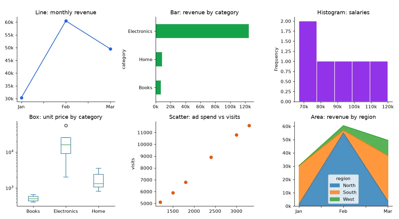
| Chart | kind= | Use it to show |
|---|---|---|
| Line | "line" | A trend over time |
| Bar | "bar", "barh" | Comparing categories; horizontal for long labels |
| Histogram | "hist" | The distribution of one numeric column |
| Box | "box" | Spread, median and outliers, compared across groups |
| Scatter | "scatter" | The relationship between two numeric columns |
| Area | "area" | How parts add up to a total over time |
| Pie | "pie" | Shares of a whole, only with a few slices; a bar chart is usually easier to read |
Matplotlib integration
.plot() returns a Matplotlib Axes, so you can customise anything Matplotlib can:
fig, ax = plt.subplots(figsize=(8, 4))
monthly.plot(ax=ax, marker="o")
ax.set_title("Monthly revenue")
ax.set_ylabel("Revenue (INR)")
ax.axhline(monthly.mean(), linestyle="--", color="grey", label="average")
ax.legend()
fig.tight_layout()
fig.savefig("monthly_revenue.png", dpi=150)
Pass ax= to place several Pandas plots in one figure, as in the grid above.
Seaborn integration
Seaborn builds statistical charts directly from long-format DataFrames:
import seaborn as sns

sns.set_theme(style="whitegrid")
sns.barplot(data=employees, x="department", y="salary", estimator="mean", errorbar=None)
sns.boxplot(data=orders, x="category", y="unit_price")
Use Pandas plotting for quick looks, Seaborn for grouped and statistical charts, and Plotly or a BI tool when people need interactive dashboards.
Chapter 17: Real-World Pandas Projects
Ten short projects that combine the earlier chapters. Each uses the sample datasets or a small inline one, so you can run them as written.
Project 1: Employee data analysis
Problem: HR wants headcount, average salary and average age per department, and the top earner in each. Input: employees.
report = (
    employees.groupby("department")
    .agg(headcount=("name", "count"), avg_salary=("salary", "mean"), avg_age=("age", "mean"))
    .round(1)
    .sort_values("avg_salary", ascending=False)
)

dept_max = employees.groupby("department")["salary"].transform("max")
top_earners = employees.loc[employees["salary"] == dept_max, ["name", "department", "salary"]]
headcount avg_salary avg_age
department
Data Science 2 98500.0 29.5
Engineering 2 97500.0 30.0
Product 1 88000.0 28.0
Sales 1 67000.0 41.0
name department salary
2 Sara Product 88000
3 Priya Engineering 120000
4 Omar Sales 67000
5 Mei Data Science 102000
How it works: named aggregation builds the summary; transform("max") puts each department's maximum next to every employee so a simple comparison finds the top earners. Business use: salary benchmarking and pay-equity reviews.
Project 2: E-commerce sales analysis
Problem: which categories drive revenue, who are the top customers, and what is the average order value? Input: orders.
cat = orders.groupby("category").agg(
    orders=("order_id", "count"), units=("quantity", "sum"), revenue=("revenue", "sum"),
)
cat["share_pct"] = (cat["revenue"] / cat["revenue"].sum() * 100).round(1)

top_customers = orders.groupby("customer_id")["revenue"].sum().nlargest(3)
aov = orders["revenue"].sum() / orders["order_id"].nunique()
orders units revenue share_pct category Electronics 5 7 124993 89.1 Home 3 6 8494 6.1 Books 4 14 6845 4.9 customer_id 2 57649 4 33993 1 31197 aov: 11694.33
Insight: Books sells the most units (14) but brings under 5% of revenue. Business use: deciding where to spend marketing budget and which customers to target for loyalty programmes.
Project 3: Customer data cleaning
Problem: a CRM export has duplicates, messy names, mixed-case emails, phone numbers in several formats and dates in two formats. Input:
   customer_id          name                 email            phone signup_date
0          101    john smith  John.Smith@Gmail.com  +91 98470-12345  2026-01-05
1          102  ALEX O'NEIL       alex@company.io       98470 55555  05/02/2026
2          103     sara khan        SARA@yahoo.com       9847011111  2026-02-10
3          103     sara khan        SARA@yahoo.com       9847011111  2026-02-10
4          104           NaN                priya@      98470 22222  2026-03-01
5          105      mei  lin   mei.lin@outlook.com              NaN   not known
def clean_customers(df: pd.DataFrame) -> tuple[pd.DataFrame, pd.DataFrame]:
    df = df.drop_duplicates(subset="customer_id").copy()
    df["name"] = df["name"].str.strip().str.replace(r"\s+", " ", regex=True).str.title()
    df["email"] = df["email"].str.strip().str.lower()
    df["phone"] = df["phone"].str.replace(r"\D", "", regex=True).str[-10:]

    iso = pd.to_datetime(df["signup_date"], format="%Y-%m-%d", errors="coerce")
    indian = pd.to_datetime(df["signup_date"], format="%d/%m/%Y", errors="coerce")
    df["signup_date"] = iso.fillna(indian)

    valid_email = df["email"].str.fullmatch(r"[\w.+-]+@[\w-]+\.[\w.]+", na=False)
    is_bad = ~valid_email | df["name"].isna()
    return df[~is_bad], df[is_bad]

good, rejected = clean_customers(raw_customers)
customer_id name email phone signup_date 0 101 John Smith john.smith@gmail.com 9847012345 2026-01-05 1 102 Alex O'Neil alex@company.io 9847055555 2026-02-05 2 103 Sara Khan sara@yahoo.com 9847011111 2026-02-10 5 105 Mei Lin mei.lin@outlook.com NaN NaT rejected: customer_id name email 4 104 NaN priya@
How it works: duplicates go first so later steps do less work. \s+ collapses double spaces; str[-10:] keeps the 10-digit mobile number after removing the country code. Each date format is parsed explicitly. Invalid rows go to a separate rejected frame instead of disappearing. Business use: CRM imports, email campaign lists, deduplicating customers before a migration.
Project 4: Monthly revenue report
monthly = orders.resample("ME", on="order_date").agg(
orders=("order_id", "count"), revenue=("revenue", "sum"),
)
monthly.index = monthly.index.strftime("%b %Y")
monthly["mom_growth_pct"] = (monthly["revenue"].pct_change() * 100).round(1)
monthly["cumulative"] = monthly["revenue"].cumsum()orders revenue mom_growth_pct cumulative order_date Jan 2026 3 30347 NaN 30347 Feb 2026 3 60493 99.3 90840 Mar 2026 6 49492 -18.2 140332
Insight: March had twice as many orders as February but 18% less revenue, because February included one 54,999 order. Order count and revenue can move in opposite directions, so report both. Business use: the monthly management report.
Project 5: Product inventory analysis
inventory = pd.DataFrame({
"sku": ["KB-01", "MS-02", "HD-03", "MN-04", "CB-05"],
"product": ["Keyboard", "Mouse", "Headset", "Monitor", "USB-C Cable"],
"stock": [12, 3, 0, 25, 140],
"reorder_level": [10, 15, 5, 8, 50],
"unit_cost": [1500, 600, 2200, 11000, 250],
"units_sold_30d": [40, 55, 18, 6, 90],
})
inventory["stock_value"] = inventory["stock"] * inventory["unit_cost"]
inventory["days_of_cover"] = (inventory["stock"] / (inventory["units_sold_30d"] / 30)).round(1)
inventory["status"] = np.select(
[inventory["stock"] == 0, inventory["stock"] <= inventory["reorder_level"]],
["out of stock", "reorder"],
default="ok",
)sku product stock stock_value days_of_cover status 0 KB-01 Keyboard 12 18000 9.0 ok 1 MS-02 Mouse 3 1800 1.6 reorder 2 HD-03 Headset 0 0 0.0 out of stock 3 MN-04 Monitor 25 275000 125.0 ok 4 CB-05 USB-C Cable 140 35000 46.7 ok
Insight: the keyboard is "ok" by its reorder level but has only 9 days of cover at the current sales rate, while monitors tie up 275,000 in stock for 125 days. Business use: purchase planning and freeing up working capital.
Project 6: Student performance analysis
students = pd.DataFrame({
"student": ["Anu", "Ben", "Chitra", "Dev", "Esha", "Farhan"],
"class": ["10A", "10A", "10A", "10B", "10B", "10B"],
"math": [78, 92, 45, 88, 67, 95],
"science": [82, 89, 52, 79, 71, 91],
"english": [91, 76, 60, 85, 74, 88],
})
subjects = ["math", "science", "english"]
students["average"] = students[subjects].mean(axis=1).round(1)
students["grade"] = pd.cut(students["average"], bins=[0, 60, 75, 90, 100],
labels=["D", "C", "B", "A"], right=False)
students["class_rank"] = students.groupby("class")["average"].rank(ascending=False, method="min").astype(int)
needs_support = students.loc[(students[subjects] < 50).any(axis=1), "student"].tolist() # ['Chitra']student class math science english average grade class_rank 0 Anu 10A 78 82 91 83.7 B 2 1 Ben 10A 92 89 76 85.7 B 1 2 Chitra 10A 45 52 60 52.3 D 3 3 Dev 10B 88 79 85 84.0 B 2 4 Esha 10B 67 71 74 70.7 C 3 5 Farhan 10B 95 91 88 91.3 A 1
mean(axis=1) averages across columns for each row. pd.cut converts scores to grade bands, and a grouped rank ranks within each class. Business use: report cards, and identifying students who need support early.
Project 7: CSV data processing
Problem: a system drops one CSV per day into a folder. Combine them, remove orders that appear in more than one file, and produce city totals.
from pathlib import Path
frames = []
for path in sorted(Path("daily_exports").glob("orders_*.csv")):
df = pd.read_csv(path)
df["source_file"] = path.name # keep lineage for debugging
frames.append(df)
combined = pd.concat(frames, ignore_index=True).drop_duplicates(subset="order_id")
combined.groupby("city", as_index=False)["amount"].sum().to_csv("city_totals.csv", index=False)order_id city amount source_file 0 1 Kochi 1200 orders_2026-03-01.csv 1 2 Chennai 800 orders_2026-03-01.csv 2 3 Kochi 450 orders_2026-03-02.csv 3 4 Delhi 2300 orders_2026-03-02.csv 4 5 Chennai 990 orders_2026-03-03.csv city_totals.csv: city,amount Chennai,1790 Delhi,2300 Kochi,1650
Order 2 appeared in two files and was counted once. Build one list and concatenate once; concatenating inside the loop copies the growing frame every time. Business use: consolidating exports from POS systems, partners or log files.
Project 8: Excel report generation
summary = orders.pivot_table(index="region", columns="category", values="revenue",
aggfunc="sum", fill_value=0, margins=True, margins_name="Total")
with pd.ExcelWriter("sales_report.xlsx", engine="openpyxl") as writer:
summary.to_excel(writer, sheet_name="Summary")
orders.to_excel(writer, sheet_name="Orders", index=False)
ws = writer.sheets["Orders"] # the openpyxl worksheet
ws.freeze_panes = "A2" # keep the header visible
for col in ws.columns: # rough auto-width
ws.column_dimensions[col[0].column_letter].width = max(len(str(c.value)) for c in col) + 2['Summary', 'Orders']
Books Electronics Home Total
region
North 2650 54999 2397 60046
South 4195 60995 0 65190
West 0 8999 6097 15096
Total 6845 124993 8494 140332
Pandas writes the data; writer.sheets exposes the underlying openpyxl worksheet for formatting. Business use: the weekly report finance asks for, generated by a scheduled job instead of by hand.
Project 9: Database data analysis
import sqlite3
conn = sqlite3.connect("shop.db") # or a SQLAlchemy engine for PostgreSQL/MySQL
customers = pd.DataFrame({"customer_id": [1, 2, 3, 4, 5, 6],
"name": ["John", "Alex", "Sara", "Priya", "Omar", "Mei"],
"city": ["Kochi", "Bengaluru", "Kochi", "Chennai", "Bengaluru", "Kochi"]})
customers.to_sql("customers", conn, index=False, if_exists="replace")
orders.to_sql("orders", conn, index=False, if_exists="replace")
query = """
SELECT c.city, o.category, o.revenue, o.order_date
FROM orders AS o
JOIN customers AS c ON c.customer_id = o.customer_id
WHERE o.order_date >= :start
"""
df = pd.read_sql(query, conn, params={"start": "2026-02-01"}, parse_dates=["order_date"])
city_report = df.pivot_table(index="city", columns="category", values="revenue",
aggfunc="sum", fill_value=0)
city_report.reset_index().to_sql("city_category_revenue", conn, index=False, if_exists="replace")category Books Electronics Home city Bengaluru 1300 54999 2598 Chennai 1995 31998 0 Kochi 2200 8999 5896
The database does the join and the date filter, where indexes help; Pandas does the reshaping, which is awkward in SQL. The result is written back as a reporting table. Business use: reporting from a production replica without adding load to the main application.
Project 10: Business KPI reporting
o = orders.copy()
o["month"] = o["order_date"].dt.to_period("M")
first_month = o.groupby("customer_id")["month"].transform("min")
o["customer_type"] = np.where(o["month"] == first_month, "new", "returning")
kpis = o.groupby("month").agg(
revenue=("revenue", "sum"),
orders=("order_id", "nunique"),
customers=("customer_id", "nunique"),
)
kpis["aov"] = (kpis["revenue"] / kpis["orders"]).round(0)
kpis["new_customers"] = o[o["customer_type"] == "new"].groupby("month")["customer_id"].nunique()
kpis["revenue_growth_pct"] = (kpis["revenue"].pct_change() * 100).round(1)
kpis["target_hit"] = kpis["revenue"] >= pd.Series([40000, 50000, 60000], index=kpis.index)revenue orders customers aov new_customers revenue_growth_pct target_hit month 2026-01 30347 3 2 10116.0 2 NaN False 2026-02 60493 3 3 20164.0 2 99.3 True 2026-03 49492 6 6 8249.0 2 -18.2 False
How it works: transform("min") finds each customer's first month, which classifies every order as new or returning. Assigning kpis["new_customers"] aligns on the month index automatically. Business use: the KPI table behind a dashboard or a board update.
Chapter 18: Performance and Best Practices
The rules that matter most
- Prefer vectorised operations. Column arithmetic ran in 0.74 ms where
apply(axis=1)took 2.64 s (Chapter 9). - Avoid loops over rows.
iterrows()was the slowest option measured. If a loop is truly unavoidable,itertuples()is much faster thaniterrows(), and a loop over NumPy arrays (df["a"].to_numpy()) faster still. - Use appropriate data types. Read IDs as strings, dates as datetimes, and numbers as numbers. Wrong types are slower and cause bugs.
- Optimise memory. Downcast numbers and load only the columns you need. Memory use went from 16.0 MB to 5.0 MB in Chapter 15.
- Use categoricals for repetitive text. 14.4 MB to 1.0 MB for a city column.
- Avoid unnecessary copies. With Copy-on-Write, extra
.copy()calls are no longer needed for safety. Do not keep five intermediate versions of a large DataFrame alive; reuse names or chain methods. - Read large files in chunks when they do not fit in memory, or convert them to Parquet once.
- Filter early. Push filters into SQL,
usecolsor Parquet reads before data reaches Pandas. - Do not grow DataFrames in a loop. Collect rows in a list and build the frame once.
- Benchmark before optimising. Guesses about performance are often wrong.
Benchmarking
# In Jupyter
%timeit df["price"] * df["qty"]
# In a script
import time
start = time.perf_counter()
result = df.groupby("region")["revenue"].sum()
print(f"{time.perf_counter() - start:.4f}s")
# Memory
df.info(memory_usage="deep")Measure on realistic data sizes. An approach that wins on 100 rows can lose on 10 million.
Readable code is a best practice too
report = (
pd.read_csv("orders.csv", parse_dates=["order_date"])
.query("region != 'West'")
.assign(month=lambda d: d["order_date"].dt.to_period("M"))
.groupby(["month", "category"], as_index=False)["revenue"].sum()
.sort_values(["month", "revenue"], ascending=[True, False])
)Method chaining reads top to bottom like a recipe, avoids half-finished intermediate variables and works naturally with Copy-on-Write. Break the chain when a step needs a comment or a check.
Testing Pandas code
import pandas.testing as pdt
def test_monthly_revenue():
result = monthly_revenue(sample_orders)
expected = pd.DataFrame({"month": ["2026-01"], "revenue": [30347]})
pdt.assert_frame_equal(result, expected)assert_frame_equal compares values, dtypes, index and column names, and prints a clear diff when they differ. Keep transformations in plain functions that take and return DataFrames, so they are easy to test with pytest. My guide on Python testing and code quality covers the rest.
When Pandas is not the right tool
Pandas works in memory on one machine. As a rough guide, it needs several times the file size in RAM while working. Its limits:
- Datasets larger than available memory.
- Many common operations use only one CPU core.
- Heavy row-by-row logic that cannot be vectorised.
- Transactional, multi-user data. That belongs in a database.
| Tool | What it is | Consider it when |
|---|---|---|
| Polars | A DataFrame library written in Rust, multi-threaded, with a lazy query optimiser | Single-machine data that is slow or tight in Pandas; new pipelines |
| DuckDB | An in-process analytical SQL database that queries Pandas frames, CSV and Parquet directly | You prefer SQL, or need joins and aggregations on larger-than-memory files |
| Dask | Parallel, chunked DataFrames with a Pandas-like API | Scaling existing Pandas code across cores or a small cluster |
| PySpark | The Python API for Apache Spark, a distributed engine | Terabyte-scale data on a cluster, often in a data platform such as Databricks |
Pandas remains the best choice for most datasets that fit in memory, thanks to its API coverage and ecosystem. Learn Pandas first; the concepts transfer directly to the others.
Chapter 19: Common Errors and Troubleshooting
| Error | Typical cause | Fix |
|---|---|---|
KeyError: 'Salary' | Column name typo, wrong case or hidden whitespace | Print df.columns.tolist(); normalise with df.columns.str.strip().str.lower() |
KeyError: 10 from .loc[10] | Label does not exist, often after filtering | Use .iloc for positions or reset_index(drop=True) |
IndexError: single positional indexer is out-of-bounds | .iloc position beyond the last row | Check len(df); handle empty results |
ValueError: Length of values (3) does not match length of index (6) | Assigning a list of the wrong length as a column | Assign a Series (aligned by index) or a list of the right length |
ValueError: The truth value of a Series is ambiguous | and/or or if on a Series; missing parentheses | Use &, |, ~ with parentheses; .any()/.all() in if |
ValueError: invalid literal for int() with base 10: 'abc' | astype(int) on dirty text | pd.to_numeric(s, errors="coerce"), then inspect the NaNs |
ChainedAssignmentError (pandas 3) / SettingWithCopyWarning (pandas 2) | df[cond]["col"] = value | df.loc[cond, "col"] = value |
ParserError: Expected 2 fields in line 3, saw 3 | Wrong delimiter, or unquoted commas inside values | Set sep; fix the export's quoting; on_bad_lines="skip" as a last resort |
FileNotFoundError | Relative path resolved from a different working directory | Build paths with Path(__file__).parent |
UnicodeDecodeError | File is not UTF-8 | encoding="latin-1" or "cp1252"; "utf-8-sig" for Excel CSVs with a BOM |
ValueError: You are trying to merge on int64 and str columns | Key types differ between frames | Convert both keys to the same type before merging |
MergeError: Merge keys are not unique | validate= caught duplicate keys | Deduplicate or aggregate the side that should be unique |
ValueError: Index contains duplicate entries, cannot reshape | pivot with duplicate index/column pairs | Use pivot_table with an aggfunc |
Silent problems (no error, wrong answer)
These are worse than exceptions, because nothing tells you something went wrong.
- Numbers stored as text.
pd.Series(["10", "20", "30"]).sum()returns'102030', string concatenation. Checkdtypesafter every read. - Row explosion after a merge. Duplicate keys on both sides multiply rows. Compare
len()before and after, and usevalidate=. - Missing values skipped in maths.
pd.Series([1, None, 3]).mean()is2.0, not 1.33, and the sum of an all-missing column is0. Decide deliberately how missing values should count. - Comparing with NaN.
== np.nanis alwaysFalse. Useisna(). - Ambiguous dates parsed in the wrong order (Chapter 13).
- Integer columns turning into floats when one value is missing; IDs then print as
101.0. UseInt64.
Performance problems
If a script is slow, check in this order: a Python loop or apply(axis=1) over rows; growing a DataFrame inside a loop; reading the same file repeatedly; text columns that should be category; and loading columns or rows that a filter later throws away.
Chapter 20: Pandas Interview Preparation
Basic questions
1. What is Pandas and what are its main data structures?
An open-source Python library for structured data. Its main structures are the Series (one-dimensional, labelled) and the DataFrame (two-dimensional, labelled rows and columns, each column a Series).
2. How do you read a CSV and inspect it?
df = pd.read_csv("file.csv"), then df.shape, df.info(), df.head() and df.describe().
3. How do you select rows where a column meets a condition?
Boolean indexing: df[df["age"] > 30]; for several conditions, df[(cond1) & (cond2)]; or df.query("age > 30").
4. How do you find and handle missing values?
df.isna().sum() to find them; fillna to replace (per-column values, ffill, interpolation) or dropna(subset=...) to remove. The right choice depends on what the column means.
5. What is the index?
The row labels. It identifies rows, drives .loc lookups and aligns data in arithmetic, joins and assignments.
Intermediate questions
6. Explain split-apply-combine.
GroupBy splits rows into groups by key, applies a function to each group (aggregate, transform or filter) and combines the results into one object.
7. What is the difference between agg and transform?
agg returns one row per group. transform returns a result the same length as the input, aligned to the original rows, so you can add a group statistic as a new column.
8. How do you remove duplicates while keeping the latest record?
df.sort_values("updated_at").drop_duplicates(subset="customer_id", keep="last").
9. How do you convert a column to datetime and get monthly totals?
df["date"] = pd.to_datetime(df["date"], format=...), then df.resample("ME", on="date")["amount"].sum().
10. How do you reshape wide data to long?
df.melt(id_vars=[...], var_name=..., value_name=...). The reverse is pivot or pivot_table.
Advanced questions
11. What is Copy-on-Write and how did pandas 3 change things?
Every derived DataFrame or Series behaves as an independent copy; data is physically copied only when one side is modified. It is the only mode in pandas 3. SettingWithCopyWarning is gone, and chained assignment (df[a][b] = x) never updates the original. Use a single .loc.
12. How would you process a 20 GB CSV on a laptop with 16 GB RAM?
Read only needed columns with explicit dtypes, process with chunksize and combine partial aggregates, or convert once to Parquet and read selected columns. If the logic needs the whole dataset (joins, medians), use DuckDB or Polars' lazy mode, or Dask.
13. Why is apply(axis=1) slow, and what do you use instead?
It calls a Python function once per row and builds a Series for each row. Replace it with vectorised column operations, np.where/np.select for conditions, pd.cut for bins, and map with a dictionary for lookups.
14. How do you reduce a DataFrame's memory?
Measure with memory_usage(deep=True), then downcast numbers, convert low-cardinality text to category, use the str or Arrow-backed types instead of object, and drop unused columns.
15. How do you replicate a SQL window function?
groupby().transform() for SUM() OVER (PARTITION BY ...), groupby().cumcount() for ROW_NUMBER(), groupby().rank() for RANK(), groupby().shift() for LAG(), and groupby().rolling() for moving windows.
Scenario-based questions
16. After merging orders with customers, your revenue total went up. Why?
The customer table has duplicate keys, so some orders matched several customer rows and were counted more than once. Check customers["customer_id"].duplicated().sum(), deduplicate, and add validate="many_to_one" to the merge.
17. A column of amounts sums to a huge string. What happened?
It was read as text, probably because of a currency symbol, thousands separator or a stray value. Clean the text and convert with pd.to_numeric(..., errors="coerce"), then investigate the rows that became NaN.
18. A daily report shows no row for days with zero sales. How do you fix it?
Use resample("D"), which includes empty periods, or reindex against pd.date_range(start, end, freq="D") with fill_value=0.
Practical coding questions
19. Top 2 earners per department
(employees.sort_values("salary", ascending=False)
.groupby("department")
.head(2))20. Percentage of each order within its region's revenue
orders["pct_of_region"] = (
orders["revenue"] / orders.groupby("region")["revenue"].transform("sum") * 100
).round(1)21. Customers who ordered in January but not in March
month = orders["order_date"].dt.month
jan = set(orders.loc[month == 1, "customer_id"])
mar = set(orders.loc[month == 3, "customer_id"])
sorted(jan - mar) # [] here: customers 1 and 2 both ordered again in March22. Second-highest salary
employees["salary"].drop_duplicates().nlargest(2).iloc[-1] # 102000Frequently asked differences
| Pair | Difference |
|---|---|
| Series vs DataFrame | One labelled column vs a table of columns sharing an index |
loc vs iloc | Labels (slice end included) vs integer positions (slice end excluded) |
merge vs join vs concat | Join on columns (default inner) vs join on the index (default left) vs stack along an axis with no key matching |
map vs apply | Series.map maps each value with a dict, Series or function; apply runs a function on values, or on rows/columns of a DataFrame |
isna vs isnull | No difference; isnull is an alias |
dropna vs fillna | Remove rows/columns with missing values vs replace missing values |
pivot vs pivot_table | Reshape only, fails on duplicates vs reshape and aggregate duplicates, with optional totals |
count vs size | Non-missing values vs all rows, including missing |
sort_values vs sort_index | Sort by column values vs sort by index labels |
Frequently Asked Questions
Is Pandas hard to learn?
The basics take a few days if you know Python: reading files, selecting, filtering, grouping. Fluency comes from using it on real, messy data. Start with the roadmap concepts, then move to groupby, merge and dates.
Do I need NumPy before learning Pandas?
No. Knowing that operations work on whole arrays at once (vectorisation) helps, and you will pick up the few NumPy functions you need, such as np.where and np.nan, along the way.
Should I learn Pandas or Polars in 2026?
Learn Pandas first. Most tutorials, libraries and existing codebases use it, and job descriptions ask for it. Polars is worth adding when performance becomes a problem; the concepts carry over directly.
How much data can Pandas handle?
As much as fits comfortably in memory, usually a few million to tens of millions of rows on a laptop. Efficient dtypes, column selection and chunking stretch that further.
Is Pandas used in backend development?
Yes: bulk imports and exports, data migrations, reports, reconciliation jobs and admin analytics. Run heavy Pandas work in background workers such as Celery rather than inside web requests.
What changed in pandas 3.0?
Copy-on-Write is always on, text columns default to the new str dtype, and deprecated APIs were removed, including DataFrame.applymap, fillna(method=...) and the "M", "Q" and "Y" frequency aliases. The official migration guide lists every change.
Conclusion
Pandas turns tabular data work into short, repeatable code. The core is small: Series and DataFrames, reading and inspecting data, selecting with loc and iloc, cleaning missing and messy values, groupby for summaries and merge for combining sources. Dates, reshaping, window functions and memory tuning build on that foundation.
Three habits matter more than any single method: vectorise instead of looping, check dtypes and row counts after every read and merge, and on pandas 3 update data with one .loc call. Pick a real CSV from your own work, run the five-minute exploration checklist from Chapter 5, and build one of the projects above on it.
Related reading
- Building Efficient Bulk CSV Import/Export and Data Migration Pipelines
- Database Optimization Guide: PostgreSQL, MySQL, SQLite and Django ORM
- Python Testing and Code Quality: Pytest, Unit Testing, Ruff and Best Practices
- Python Concurrency for Backend Developers: Threads, asyncio and Processes
Further Learning Resources
- Pandas Roadmap (PDF carousel): my 12-slide visual summary of the 10 essential concepts, a good companion to this article
- pandas documentation: the user guide and API reference
- 10 minutes to pandas: the official quick tour
- Copy-on-Write (CoW): the official explanation of the pandas 3 behaviour
- Migration guide for the new string data type
- Comparison with SQL: SQL queries and their Pandas equivalents
- Python for Data Analysis by Wes McKinney, the creator of Pandas, free to read online